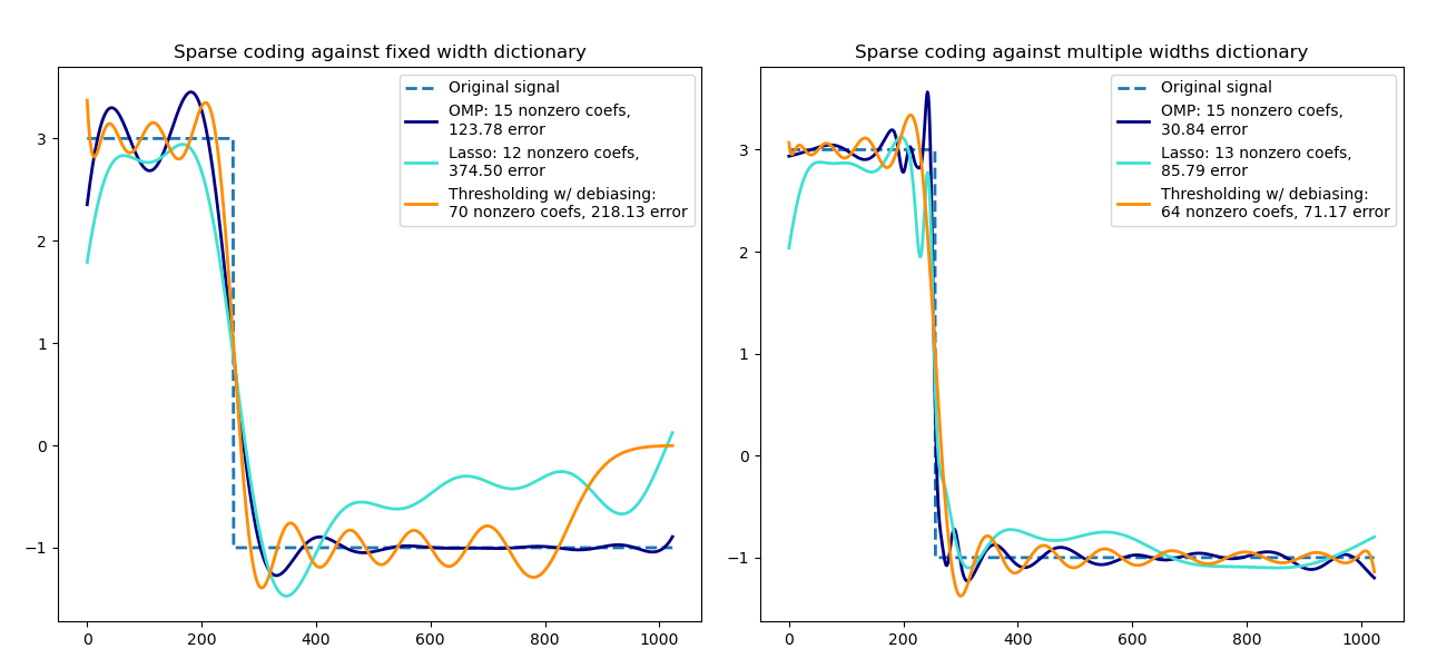
Sparse Kodierung mit einem vorab berechneten Dictionary

Transformieren Sie ein Signal als eine spärliche Kombination von Ricker-Wavelets. Dieses Beispiel vergleicht visuell verschiedene Sparse-Coding-Methoden unter Verwendung des SparseCoder-Schätzers. Das Ricker-Wavelet (auch bekannt als Mexican Hat oder die zweite Ableitung eines Gaußschen) ist kein besonders guter Kern, um stückweise konstante Signale wie dieses darzustellen. Es kann daher gezeigt werden, wie wichtig es ist, verschiedene Breiten von Atomen hinzuzufügen, und motiviert daher das Erlernen des Dictionarys, um Ihren Signaltyp am besten anzupassen.

Das reichhaltigere Dictionary auf der rechten Seite ist nicht größer; es wird ein stärkeres Subsampling durchgeführt, um in derselben Größenordnung zu bleiben.

# Authors: The scikit-learn developers
# SPDX-License-Identifier: BSD-3-Clause

import matplotlib.pyplot as plt
import numpy as np

from sklearn.decomposition import SparseCoder


def ricker_function(resolution, center, width):
    """Discrete sub-sampled Ricker (Mexican hat) wavelet"""
    x = np.linspace(0, resolution - 1, resolution)
    x = (
        (2 / (np.sqrt(3 * width) * np.pi**0.25))
        * (1 - (x - center) ** 2 / width**2)
        * np.exp(-((x - center) ** 2) / (2 * width**2))
    )
    return x


def ricker_matrix(width, resolution, n_components):
    """Dictionary of Ricker (Mexican hat) wavelets"""
    centers = np.linspace(0, resolution - 1, n_components)
    D = np.empty((n_components, resolution))
    for i, center in enumerate(centers):
        D[i] = ricker_function(resolution, center, width)
    D /= np.sqrt(np.sum(D**2, axis=1))[:, np.newaxis]
    return D


resolution = 1024
subsampling = 3  # subsampling factor
width = 100
n_components = resolution // subsampling

# Compute a wavelet dictionary
D_fixed = ricker_matrix(width=width, resolution=resolution, n_components=n_components)
D_multi = np.r_[
    tuple(
        ricker_matrix(width=w, resolution=resolution, n_components=n_components // 5)
        for w in (10, 50, 100, 500, 1000)
    )
]

# Generate a signal
y = np.linspace(0, resolution - 1, resolution)
first_quarter = y < resolution / 4
y[first_quarter] = 3.0
y[np.logical_not(first_quarter)] = -1.0

# List the different sparse coding methods in the following format:
# (title, transform_algorithm, transform_alpha,
#  transform_n_nozero_coefs, color)
estimators = [
    ("OMP", "omp", None, 15, "navy"),
    ("Lasso", "lasso_lars", 2, None, "turquoise"),
]
lw = 2

plt.figure(figsize=(13, 6))
for subplot, (D, title) in enumerate(
    zip((D_fixed, D_multi), ("fixed width", "multiple widths"))
):
    plt.subplot(1, 2, subplot + 1)
    plt.title("Sparse coding against %s dictionary" % title)
    plt.plot(y, lw=lw, linestyle="--", label="Original signal")
    # Do a wavelet approximation
    for title, algo, alpha, n_nonzero, color in estimators:
        coder = SparseCoder(
            dictionary=D,
            transform_n_nonzero_coefs=n_nonzero,
            transform_alpha=alpha,
            transform_algorithm=algo,
        )
        x = coder.transform(y.reshape(1, -1))
        density = len(np.flatnonzero(x))
        x = np.ravel(np.dot(x, D))
        squared_error = np.sum((y - x) ** 2)
        plt.plot(
            x,
            color=color,
            lw=lw,
            label="%s: %s nonzero coefs,\n%.2f error" % (title, density, squared_error),
        )

    # Soft thresholding debiasing
    coder = SparseCoder(
        dictionary=D, transform_algorithm="threshold", transform_alpha=20
    )
    x = coder.transform(y.reshape(1, -1))
    _, idx = (x != 0).nonzero()
    x[0, idx], _, _, _ = np.linalg.lstsq(D[idx, :].T, y, rcond=None)
    x = np.ravel(np.dot(x, D))
    squared_error = np.sum((y - x) ** 2)
    plt.plot(
        x,
        color="darkorange",
        lw=lw,
        label="Thresholding w/ debiasing:\n%d nonzero coefs, %.2f error"
        % (len(idx), squared_error),
    )
    plt.axis("tight")
    plt.legend(shadow=False, loc="best")
plt.subplots_adjust(0.04, 0.07, 0.97, 0.90, 0.09, 0.2)
plt.show()

Verwandte Beispiele

Orthogonal Matching Pursuit

Orthogonal Matching Pursuit

Zerlegung von Gesicht-Datensätzen

Zerlegung von Gesicht-Datensätzen

SGD: konvexe Verlustfunktionen

SGD: konvexe Verlustfunktionen

Bildrauschen mit Dictionary Learning

Bildrauschen mit Dictionary Learning