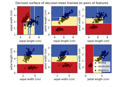
Visualisierung der Entscheidungsflächen von Baum-Ensembles im Iris-Datensatz

Visualisierung der Entscheidungsflächen von Wäldern zufälliger Bäume, trainiert auf Paaren von Merkmalen des Iris-Datensatzes.

Diese Abbildung vergleicht die Entscheidungsflächen, die von einem Entscheidungsbaum-Klassifikator (erste Spalte), einem Random Forest-Klassifikator (zweite Spalte), einem Extra-Trees-Klassifikator (dritte Spalte) und einem AdaBoost-Klassifikator (vierte Spalte) gelernt wurden.

In der ersten Zeile werden die Klassifikatoren nur anhand der Merkmale "Sepal width" und "Sepal length" gebildet, in der zweiten Zeile nur anhand von "Petal length" und "Sepal length" und in der dritten Zeile nur anhand von "Petal width" und "Petal length".

In absteigender Reihenfolge der Qualität, wenn sie (außerhalb dieses Beispiels) auf allen 4 Merkmalen mit 30 Schätzern trainiert und mittels 10-facher Kreuzvalidierung bewertet werden, sehen wir

ExtraTreesClassifier()  # 0.95 score
RandomForestClassifier()  # 0.94 score
AdaBoost(DecisionTree(max_depth=3))  # 0.94 score
DecisionTree(max_depth=None)  # 0.94 score

Das Erhöhen von max_depth für AdaBoost senkt die Standardabweichung der Scores (aber der durchschnittliche Score verbessert sich nicht).

Siehe die Konsolenausgabe für weitere Details zu jedem Modell.

In diesem Beispiel könnten Sie versuchen,

1. die max_depth für den DecisionTreeClassifier und AdaBoostClassifier zu variieren, vielleicht max_depth=3 für den DecisionTreeClassifier oder max_depth=None für AdaBoostClassifier ausprobieren

2. die n_estimators zu variieren

Es ist erwähnenswert, dass RandomForests und ExtraTrees parallel auf vielen Kernen angepasst werden können, da jeder Baum unabhängig von den anderen aufgebaut wird. Die Samples von AdaBoost werden sequenziell aufgebaut und nutzen daher keine mehreren Kerne.

DecisionTree with features [0, 1] has a score of 0.9266666666666666
RandomForest with 30 estimators with features [0, 1] has a score of 0.9266666666666666
ExtraTrees with 30 estimators with features [0, 1] has a score of 0.9266666666666666
AdaBoost with 30 estimators with features [0, 1] has a score of 0.82
DecisionTree with features [0, 2] has a score of 0.9933333333333333
RandomForest with 30 estimators with features [0, 2] has a score of 0.9933333333333333
ExtraTrees with 30 estimators with features [0, 2] has a score of 0.9933333333333333
AdaBoost with 30 estimators with features [0, 2] has a score of 0.9933333333333333
DecisionTree with features [2, 3] has a score of 0.9933333333333333
RandomForest with 30 estimators with features [2, 3] has a score of 0.9933333333333333
ExtraTrees with 30 estimators with features [2, 3] has a score of 0.9933333333333333
AdaBoost with 30 estimators with features [2, 3] has a score of 0.9866666666666667

# Authors: The scikit-learn developers
# SPDX-License-Identifier: BSD-3-Clause

import matplotlib.pyplot as plt
import numpy as np
from matplotlib.colors import ListedColormap

from sklearn.datasets import load_iris
from sklearn.ensemble import (
    AdaBoostClassifier,
    ExtraTreesClassifier,
    RandomForestClassifier,
)
from sklearn.tree import DecisionTreeClassifier

# Parameters
n_classes = 3
n_estimators = 30
cmap = plt.cm.RdYlBu
plot_step = 0.02  # fine step width for decision surface contours
plot_step_coarser = 0.5  # step widths for coarse classifier guesses
RANDOM_SEED = 13  # fix the seed on each iteration

# Load data
iris = load_iris()

plot_idx = 1

models = [
    DecisionTreeClassifier(max_depth=None),
    RandomForestClassifier(n_estimators=n_estimators),
    ExtraTreesClassifier(n_estimators=n_estimators),
    AdaBoostClassifier(DecisionTreeClassifier(max_depth=3), n_estimators=n_estimators),
]

for pair in ([0, 1], [0, 2], [2, 3]):
    for model in models:
        # We only take the two corresponding features
        X = iris.data[:, pair]
        y = iris.target

        # Shuffle
        idx = np.arange(X.shape[0])
        np.random.seed(RANDOM_SEED)
        np.random.shuffle(idx)
        X = X[idx]
        y = y[idx]

        # Standardize
        mean = X.mean(axis=0)
        std = X.std(axis=0)
        X = (X - mean) / std

        # Train
        model.fit(X, y)

        scores = model.score(X, y)
        # Create a title for each column and the console by using str() and
        # slicing away useless parts of the string
        model_title = str(type(model)).split(".")[-1][:-2][: -len("Classifier")]

        model_details = model_title
        if hasattr(model, "estimators_"):
            model_details += " with {} estimators".format(len(model.estimators_))
        print(model_details + " with features", pair, "has a score of", scores)

        plt.subplot(3, 4, plot_idx)
        if plot_idx <= len(models):
            # Add a title at the top of each column
            plt.title(model_title, fontsize=9)

        # Now plot the decision boundary using a fine mesh as input to a
        # filled contour plot
        x_min, x_max = X[:, 0].min() - 1, X[:, 0].max() + 1
        y_min, y_max = X[:, 1].min() - 1, X[:, 1].max() + 1
        xx, yy = np.meshgrid(
            np.arange(x_min, x_max, plot_step), np.arange(y_min, y_max, plot_step)
        )

        # Plot either a single DecisionTreeClassifier or alpha blend the
        # decision surfaces of the ensemble of classifiers
        if isinstance(model, DecisionTreeClassifier):
            Z = model.predict(np.c_[xx.ravel(), yy.ravel()])
            Z = Z.reshape(xx.shape)
            cs = plt.contourf(xx, yy, Z, cmap=cmap)
        else:
            # Choose alpha blend level with respect to the number
            # of estimators
            # that are in use (noting that AdaBoost can use fewer estimators
            # than its maximum if it achieves a good enough fit early on)
            estimator_alpha = 1.0 / len(model.estimators_)
            for tree in model.estimators_:
                Z = tree.predict(np.c_[xx.ravel(), yy.ravel()])
                Z = Z.reshape(xx.shape)
                cs = plt.contourf(xx, yy, Z, alpha=estimator_alpha, cmap=cmap)

        # Build a coarser grid to plot a set of ensemble classifications
        # to show how these are different to what we see in the decision
        # surfaces. These points are regularly space and do not have a
        # black outline
        xx_coarser, yy_coarser = np.meshgrid(
            np.arange(x_min, x_max, plot_step_coarser),
            np.arange(y_min, y_max, plot_step_coarser),
        )
        Z_points_coarser = model.predict(
            np.c_[xx_coarser.ravel(), yy_coarser.ravel()]
        ).reshape(xx_coarser.shape)
        cs_points = plt.scatter(
            xx_coarser,
            yy_coarser,
            s=15,
            c=Z_points_coarser,
            cmap=cmap,
            edgecolors="none",
        )

        # Plot the training points, these are clustered together and have a
        # black outline
        plt.scatter(
            X[:, 0],
            X[:, 1],
            c=y,
            cmap=ListedColormap(["r", "y", "b"]),
            edgecolor="k",
            s=20,
        )
        plot_idx += 1  # move on to the next plot in sequence

plt.suptitle("Classifiers on feature subsets of the Iris dataset", fontsize=12)
plt.axis("tight")
plt.tight_layout(h_pad=0.2, w_pad=0.2, pad=2.5)
plt.show()

Verwandte Beispiele

Gauß-Prozess-Klassifikation (GPC) auf dem Iris-Datensatz

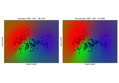
Gauß-Prozess-Klassifikation (GPC) auf dem Iris-Datensatz

Variierende Regularisierung im Multi-Layer Perceptron

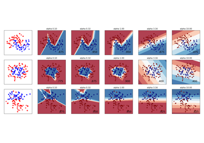
Variierende Regularisierung im Multi-Layer Perceptron

Entscheidungsfläche von Entscheidungsbäumen, trainiert auf dem Iris-Datensatz, plotten

Entscheidungsfläche von Entscheidungsbäumen, trainiert auf dem Iris-Datensatz, plotten

SGD: Gewichtete Stichproben

SGD: Gewichtete Stichproben