One-Class SVM im Vergleich zu One-Class SVM mit stochastischem Gradientenabstieg

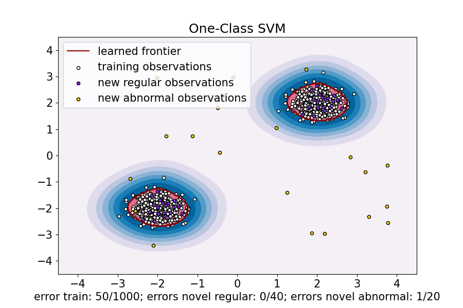
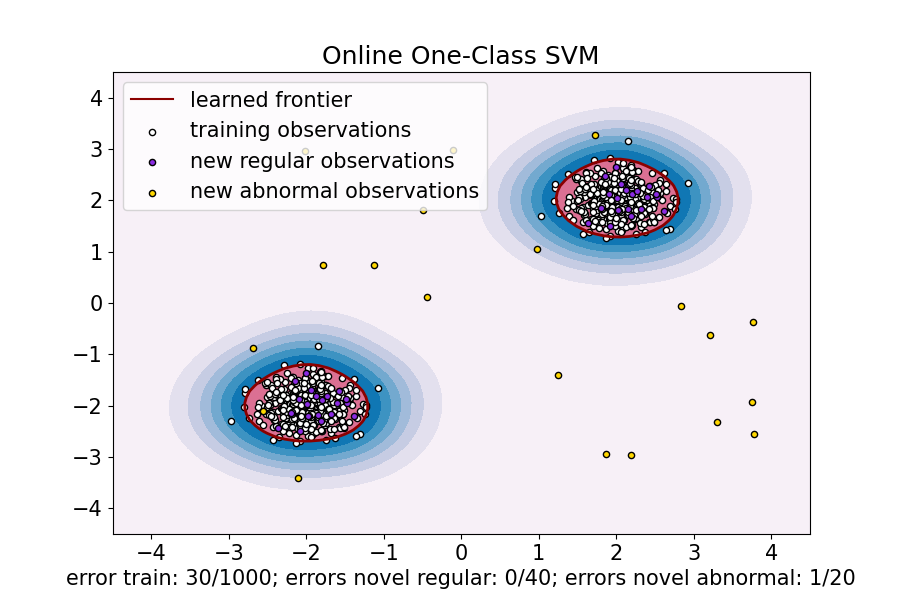
Dieses Beispiel zeigt, wie die Lösung von sklearn.svm.OneClassSVM im Falle eines RBF-Kernels mit sklearn.linear_model.SGDOneClassSVM, einer Version des One-Class SVM mit stochastischem Gradientenabstieg (SGD), angenähert werden kann. Zuerst wird eine Kernel-Approximation verwendet, um sklearn.linear_model.SGDOneClassSVM anzuwenden, das einen linearen One-Class SVM mit SGD implementiert.

Beachten Sie, dass sklearn.linear_model.SGDOneClassSVM linear mit der Anzahl der Stichproben skaliert, während die Komplexität eines kernelisierten sklearn.svm.OneClassSVM im besten Fall quadratisch zur Anzahl der Stichproben ist. Es ist nicht der Zweck dieses Beispiels, die Vorteile einer solchen Approximation in Bezug auf die Rechenzeit zu veranschaulichen, sondern vielmehr zu zeigen, dass wir auf einem einfachen Datensatz ähnliche Ergebnisse erzielen.

# Authors: The scikit-learn developers
# SPDX-License-Identifier: BSD-3-Clause

import matplotlib
import matplotlib.lines as mlines
import matplotlib.pyplot as plt
import numpy as np

from sklearn.kernel_approximation import Nystroem
from sklearn.linear_model import SGDOneClassSVM
from sklearn.pipeline import make_pipeline
from sklearn.svm import OneClassSVM

font = {"weight": "normal", "size": 15}

matplotlib.rc("font", **font)

random_state = 42
rng = np.random.RandomState(random_state)

# Generate train data
X = 0.3 * rng.randn(500, 2)
X_train = np.r_[X + 2, X - 2]
# Generate some regular novel observations
X = 0.3 * rng.randn(20, 2)
X_test = np.r_[X + 2, X - 2]
# Generate some abnormal novel observations
X_outliers = rng.uniform(low=-4, high=4, size=(20, 2))

# OCSVM hyperparameters
nu = 0.05
gamma = 2.0

# Fit the One-Class SVM
clf = OneClassSVM(gamma=gamma, kernel="rbf", nu=nu)
clf.fit(X_train)
y_pred_train = clf.predict(X_train)
y_pred_test = clf.predict(X_test)
y_pred_outliers = clf.predict(X_outliers)
n_error_train = y_pred_train[y_pred_train == -1].size
n_error_test = y_pred_test[y_pred_test == -1].size
n_error_outliers = y_pred_outliers[y_pred_outliers == 1].size

# Fit the One-Class SVM using a kernel approximation and SGD
transform = Nystroem(gamma=gamma, random_state=random_state)
clf_sgd = SGDOneClassSVM(
    nu=nu, shuffle=True, fit_intercept=True, random_state=random_state, tol=1e-4
)
pipe_sgd = make_pipeline(transform, clf_sgd)
pipe_sgd.fit(X_train)
y_pred_train_sgd = pipe_sgd.predict(X_train)
y_pred_test_sgd = pipe_sgd.predict(X_test)
y_pred_outliers_sgd = pipe_sgd.predict(X_outliers)
n_error_train_sgd = y_pred_train_sgd[y_pred_train_sgd == -1].size
n_error_test_sgd = y_pred_test_sgd[y_pred_test_sgd == -1].size
n_error_outliers_sgd = y_pred_outliers_sgd[y_pred_outliers_sgd == 1].size

from sklearn.inspection import DecisionBoundaryDisplay

_, ax = plt.subplots(figsize=(9, 6))

xx, yy = np.meshgrid(np.linspace(-4.5, 4.5, 50), np.linspace(-4.5, 4.5, 50))
X = np.concatenate([xx.ravel().reshape(-1, 1), yy.ravel().reshape(-1, 1)], axis=1)
DecisionBoundaryDisplay.from_estimator(
    clf,
    X,
    response_method="decision_function",
    plot_method="contourf",
    ax=ax,
    cmap="PuBu",
)
DecisionBoundaryDisplay.from_estimator(
    clf,
    X,
    response_method="decision_function",
    plot_method="contour",
    ax=ax,
    linewidths=2,
    colors="darkred",
    levels=[0],
)
DecisionBoundaryDisplay.from_estimator(
    clf,
    X,
    response_method="decision_function",
    plot_method="contourf",
    ax=ax,
    colors="palevioletred",
    levels=[0, clf.decision_function(X).max()],
)

s = 20
b1 = plt.scatter(X_train[:, 0], X_train[:, 1], c="white", s=s, edgecolors="k")
b2 = plt.scatter(X_test[:, 0], X_test[:, 1], c="blueviolet", s=s, edgecolors="k")
c = plt.scatter(X_outliers[:, 0], X_outliers[:, 1], c="gold", s=s, edgecolors="k")

ax.set(
    title="One-Class SVM",
    xlim=(-4.5, 4.5),
    ylim=(-4.5, 4.5),
    xlabel=(
        f"error train: {n_error_train}/{X_train.shape[0]}; "
        f"errors novel regular: {n_error_test}/{X_test.shape[0]}; "
        f"errors novel abnormal: {n_error_outliers}/{X_outliers.shape[0]}"
    ),
)
_ = ax.legend(
    [mlines.Line2D([], [], color="darkred", label="learned frontier"), b1, b2, c],
    [
        "learned frontier",
        "training observations",
        "new regular observations",
        "new abnormal observations",
    ],
    loc="upper left",
)

_, ax = plt.subplots(figsize=(9, 6))

xx, yy = np.meshgrid(np.linspace(-4.5, 4.5, 50), np.linspace(-4.5, 4.5, 50))
X = np.concatenate([xx.ravel().reshape(-1, 1), yy.ravel().reshape(-1, 1)], axis=1)
DecisionBoundaryDisplay.from_estimator(
    pipe_sgd,
    X,
    response_method="decision_function",
    plot_method="contourf",
    ax=ax,
    cmap="PuBu",
)
DecisionBoundaryDisplay.from_estimator(
    pipe_sgd,
    X,
    response_method="decision_function",
    plot_method="contour",
    ax=ax,
    linewidths=2,
    colors="darkred",
    levels=[0],
)
DecisionBoundaryDisplay.from_estimator(
    pipe_sgd,
    X,
    response_method="decision_function",
    plot_method="contourf",
    ax=ax,
    colors="palevioletred",
    levels=[0, pipe_sgd.decision_function(X).max()],
)

s = 20
b1 = plt.scatter(X_train[:, 0], X_train[:, 1], c="white", s=s, edgecolors="k")
b2 = plt.scatter(X_test[:, 0], X_test[:, 1], c="blueviolet", s=s, edgecolors="k")
c = plt.scatter(X_outliers[:, 0], X_outliers[:, 1], c="gold", s=s, edgecolors="k")

ax.set(
    title="Online One-Class SVM",
    xlim=(-4.5, 4.5),
    ylim=(-4.5, 4.5),
    xlabel=(
        f"error train: {n_error_train_sgd}/{X_train.shape[0]}; "
        f"errors novel regular: {n_error_test_sgd}/{X_test.shape[0]}; "
        f"errors novel abnormal: {n_error_outliers_sgd}/{X_outliers.shape[0]}"
    ),
)
ax.legend(
    [mlines.Line2D([], [], color="darkred", label="learned frontier"), b1, b2, c],
    [
        "learned frontier",
        "training observations",
        "new regular observations",
        "new abnormal observations",
    ],
    loc="upper left",
)
plt.show()

Verwandte Beispiele

One-Class SVM mit nicht-linearem Kernel (RBF)

One-Class SVM mit nicht-linearem Kernel (RBF)

Neuartigkeitserkennung mit Local Outlier Factor (LOF)

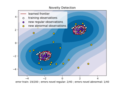
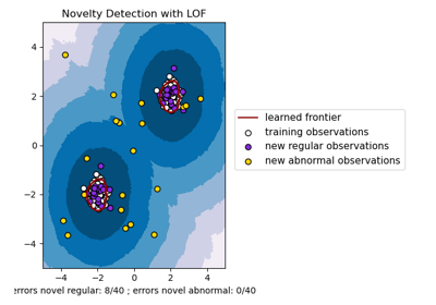
Neuartigkeitserkennung mit Local Outlier Factor (LOF)

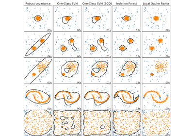
Vergleich von Anomalieerkennungsalgorithmen zur Ausreißererkennung auf Toy-Datensätzen

Vergleich von Anomalieerkennungsalgorithmen zur Ausreißererkennung auf Toy-Datensätzen

SVM-Randbeispiel

SVM-Randbeispiel