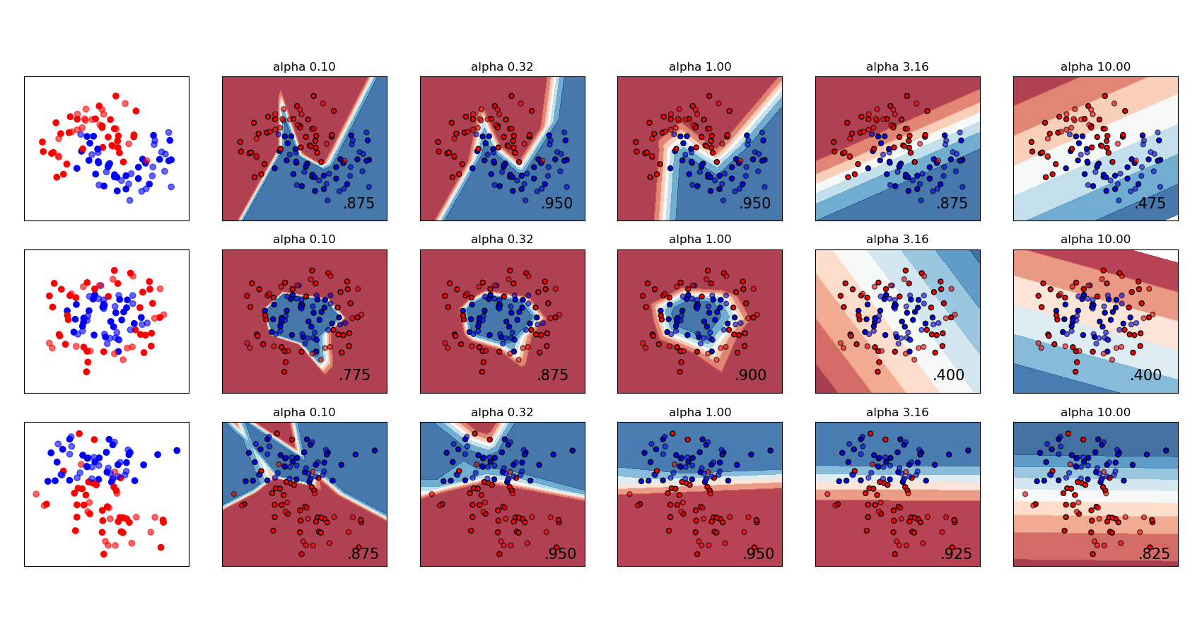
Variierende Regularisierung in Multi-layer Perceptron

Ein Vergleich verschiedener Werte für den Regularisierungsparameter „alpha“ auf synthetischen Datensätzen. Die Grafik zeigt, dass unterschiedliche Alphas unterschiedliche Entscheidungsfunktionen ergeben.

Alpha ist ein Parameter für den Regularisierungsterm, auch Strafterm genannt, der Überanpassung bekämpft, indem die Größe der Gewichte eingeschränkt wird. Ein Erhöhen von Alpha kann hohe Varianz (ein Zeichen von Überanpassung) beheben, indem kleinere Gewichte gefördert werden, was zu einem Entscheidungsflächen-Diagramm mit geringeren Krümmungen führt. Ebenso kann ein Verringern von Alpha hohe Bias (ein Zeichen von Unteranpassung) beheben, indem größere Gewichte gefördert werden, was potenziell zu einer komplizierteren Entscheidungsfläche führt.

# Authors: The scikit-learn developers
# SPDX-License-Identifier: BSD-3-Clause

import numpy as np
from matplotlib import pyplot as plt
from matplotlib.colors import ListedColormap

from sklearn.datasets import make_circles, make_classification, make_moons
from sklearn.model_selection import train_test_split
from sklearn.neural_network import MLPClassifier
from sklearn.pipeline import make_pipeline
from sklearn.preprocessing import StandardScaler

h = 0.02  # step size in the mesh

alphas = np.logspace(-1, 1, 5)

classifiers = []
names = []
for alpha in alphas:
    classifiers.append(
        make_pipeline(
            StandardScaler(),
            MLPClassifier(
                solver="lbfgs",
                alpha=alpha,
                random_state=1,
                max_iter=2000,
                early_stopping=True,
                hidden_layer_sizes=[10, 10],
            ),
        )
    )
    names.append(f"alpha {alpha:.2f}")

X, y = make_classification(
    n_features=2, n_redundant=0, n_informative=2, random_state=0, n_clusters_per_class=1
)
rng = np.random.RandomState(2)
X += 2 * rng.uniform(size=X.shape)
linearly_separable = (X, y)

datasets = [
    make_moons(noise=0.3, random_state=0),
    make_circles(noise=0.2, factor=0.5, random_state=1),
    linearly_separable,
]

figure = plt.figure(figsize=(17, 9))
i = 1
# iterate over datasets
for X, y in datasets:
    # split into training and test part
    X_train, X_test, y_train, y_test = train_test_split(
        X, y, test_size=0.4, random_state=42
    )

    x_min, x_max = X[:, 0].min() - 0.5, X[:, 0].max() + 0.5
    y_min, y_max = X[:, 1].min() - 0.5, X[:, 1].max() + 0.5
    xx, yy = np.meshgrid(np.arange(x_min, x_max, h), np.arange(y_min, y_max, h))

    # just plot the dataset first
    cm = plt.cm.RdBu
    cm_bright = ListedColormap(["#FF0000", "#0000FF"])
    ax = plt.subplot(len(datasets), len(classifiers) + 1, i)
    # Plot the training points
    ax.scatter(X_train[:, 0], X_train[:, 1], c=y_train, cmap=cm_bright)
    # and testing points
    ax.scatter(X_test[:, 0], X_test[:, 1], c=y_test, cmap=cm_bright, alpha=0.6)
    ax.set_xlim(xx.min(), xx.max())
    ax.set_ylim(yy.min(), yy.max())
    ax.set_xticks(())
    ax.set_yticks(())
    i += 1

    # iterate over classifiers
    for name, clf in zip(names, classifiers):
        ax = plt.subplot(len(datasets), len(classifiers) + 1, i)
        clf.fit(X_train, y_train)
        score = clf.score(X_test, y_test)

        # Plot the decision boundary. For that, we will assign a color to each
        # point in the mesh [x_min, x_max] x [y_min, y_max].
        if hasattr(clf, "decision_function"):
            Z = clf.decision_function(np.column_stack([xx.ravel(), yy.ravel()]))
        else:
            Z = clf.predict_proba(np.column_stack([xx.ravel(), yy.ravel()]))[:, 1]

        # Put the result into a color plot
        Z = Z.reshape(xx.shape)
        ax.contourf(xx, yy, Z, cmap=cm, alpha=0.8)

        # Plot also the training points
        ax.scatter(
            X_train[:, 0],
            X_train[:, 1],
            c=y_train,
            cmap=cm_bright,
            edgecolors="black",
            s=25,
        )
        # and testing points
        ax.scatter(
            X_test[:, 0],
            X_test[:, 1],
            c=y_test,
            cmap=cm_bright,
            alpha=0.6,
            edgecolors="black",
            s=25,
        )

        ax.set_xlim(xx.min(), xx.max())
        ax.set_ylim(yy.min(), yy.max())
        ax.set_xticks(())
        ax.set_yticks(())
        ax.set_title(name)
        ax.text(
            xx.max() - 0.3,
            yy.min() + 0.3,
            f"{score:.3f}".lstrip("0"),
            size=15,
            horizontalalignment="right",
        )
        i += 1

figure.subplots_adjust(left=0.02, right=0.98)
plt.show()

Verwandte Beispiele

Merkmalsdiskretisierung

Merkmalsdiskretisierung

Klassifikator-Vergleich

Klassifikator-Vergleich

Gauß-Prozess-Klassifikation (GPC) auf dem Iris-Datensatz

Gauß-Prozess-Klassifikation (GPC) auf dem Iris-Datensatz

SVM-Randbeispiel

SVM-Randbeispiel