Manifold Learning-Methoden auf einer aufgeschnittenen Sphäre

Eine Anwendung der verschiedenen Manifold Learning-Techniken auf einem sphärischen Datensatz. Hier kann man die Verwendung der Dimensionsreduktion sehen, um etwas Intuition bezüglich der Manifold Learning-Methoden zu gewinnen. Bezüglich des Datensatzes sind die Pole von der Sphäre abgeschnitten, ebenso wie ein dünner Streifen an der Seite. Dies ermöglicht es den Manifold Learning-Techniken, sie „aufzuklappen“, während sie auf zwei Dimensionen projiziert wird.

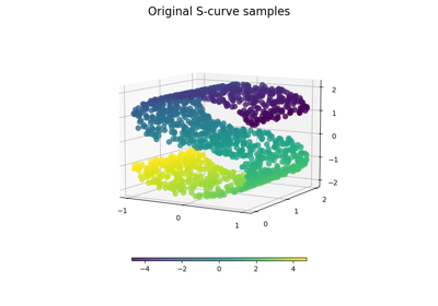
Für ein ähnliches Beispiel, bei dem die Methoden auf dem S-Kurven-Datensatz angewendet werden, siehe Vergleich von Manifold Learning-Methoden.

Beachte, dass der Zweck von MDS darin besteht, eine niedrigdimensionale Darstellung der Daten (hier 2D) zu finden, bei der die Abstände die Abstände im ursprünglichen hochdimensionalen Raum gut widerspiegeln. Im Gegensatz zu anderen Manifold Learning-Algorithmen versucht es nicht, eine isotrope Darstellung der Daten im niedrigdimensionalen Raum zu erzielen. Hier entspricht das Manifold-Problem ziemlich der Darstellung einer flachen Karte der Erde, wie bei der Kartenprojektion.

standard: 0.06 sec
ltsa: 0.8 sec
hessian: 0.69 sec
modified: 1.2 sec
ISO: 0.1 sec
MDS: 0.89 sec
Non-metric MDS: 11 sec
Classical MDS: 0.039 sec
Spectral Embedding: 0.041 sec
t-SNE: 3.7 sec

# Authors: The scikit-learn developers
# SPDX-License-Identifier: BSD-3-Clause

from time import time

import matplotlib.pyplot as plt

# Unused but required import for doing 3d projections with matplotlib < 3.2
import mpl_toolkits.mplot3d  # noqa: F401
import numpy as np
from matplotlib.ticker import NullFormatter

from sklearn import manifold
from sklearn.utils import check_random_state

# Variables for manifold learning.
n_neighbors = 10
n_samples = 1000

# Create our sphere.
random_state = check_random_state(0)
p = random_state.rand(n_samples) * (2 * np.pi - 0.55)
t = random_state.rand(n_samples) * np.pi

# Sever the poles from the sphere.
indices = (t < (np.pi - (np.pi / 8))) & (t > (np.pi / 8))
colors = p[indices]
x, y, z = (
    np.sin(t[indices]) * np.cos(p[indices]),
    np.sin(t[indices]) * np.sin(p[indices]),
    np.cos(t[indices]),
)

# Plot our dataset.
fig = plt.figure(figsize=(15, 12))
plt.suptitle(
    "Manifold Learning with %i points, %i neighbors" % (1000, n_neighbors), fontsize=14
)

ax = fig.add_subplot(351, projection="3d")
ax.scatter(x, y, z, c=p[indices], cmap=plt.cm.rainbow)
ax.view_init(40, -10)

sphere_data = np.array([x, y, z]).T

# Perform Locally Linear Embedding Manifold learning
methods = ["standard", "ltsa", "hessian", "modified"]
labels = ["LLE", "LTSA", "Hessian LLE", "Modified LLE"]

for i, method in enumerate(methods):
    t0 = time()
    trans_data = (
        manifold.LocallyLinearEmbedding(
            n_neighbors=n_neighbors, n_components=2, method=method, random_state=42
        )
        .fit_transform(sphere_data)
        .T
    )
    t1 = time()
    print("%s: %.2g sec" % (methods[i], t1 - t0))

    ax = fig.add_subplot(352 + i)
    plt.scatter(trans_data[0], trans_data[1], c=colors, cmap=plt.cm.rainbow)
    plt.title("%s (%.2g sec)" % (labels[i], t1 - t0))
    ax.xaxis.set_major_formatter(NullFormatter())
    ax.yaxis.set_major_formatter(NullFormatter())
    plt.axis("tight")

# Perform Isomap Manifold learning.
t0 = time()
trans_data = (
    manifold.Isomap(n_neighbors=n_neighbors, n_components=2)
    .fit_transform(sphere_data)
    .T
)
t1 = time()
print("%s: %.2g sec" % ("ISO", t1 - t0))

ax = fig.add_subplot(357)
plt.scatter(trans_data[0], trans_data[1], c=colors, cmap=plt.cm.rainbow)
plt.title("%s (%.2g sec)" % ("Isomap", t1 - t0))
ax.xaxis.set_major_formatter(NullFormatter())
ax.yaxis.set_major_formatter(NullFormatter())
plt.axis("tight")

# Perform Multi-dimensional scaling.
t0 = time()
mds = manifold.MDS(2, n_init=1, random_state=42, init="classical_mds")
trans_data = mds.fit_transform(sphere_data).T
t1 = time()
print("MDS: %.2g sec" % (t1 - t0))

ax = fig.add_subplot(358)
plt.scatter(trans_data[0], trans_data[1], c=colors, cmap=plt.cm.rainbow)
plt.title("MDS (%.2g sec)" % (t1 - t0))
ax.xaxis.set_major_formatter(NullFormatter())
ax.yaxis.set_major_formatter(NullFormatter())
plt.axis("tight")

t0 = time()
mds = manifold.MDS(2, n_init=1, random_state=42, metric_mds=False, init="classical_mds")
trans_data = mds.fit_transform(sphere_data).T
t1 = time()
print("Non-metric MDS: %.2g sec" % (t1 - t0))

ax = fig.add_subplot(359)
plt.scatter(trans_data[0], trans_data[1], c=colors, cmap=plt.cm.rainbow)
plt.title("Non-metric MDS (%.2g sec)" % (t1 - t0))
ax.xaxis.set_major_formatter(NullFormatter())
ax.yaxis.set_major_formatter(NullFormatter())
plt.axis("tight")

t0 = time()
mds = manifold.ClassicalMDS(2)
trans_data = mds.fit_transform(sphere_data).T
t1 = time()
print("Classical MDS: %.2g sec" % (t1 - t0))

ax = fig.add_subplot(3, 5, 10)
plt.scatter(trans_data[0], trans_data[1], c=colors, cmap=plt.cm.rainbow)
plt.title("Classical MDS (%.2g sec)" % (t1 - t0))
ax.xaxis.set_major_formatter(NullFormatter())
ax.yaxis.set_major_formatter(NullFormatter())
plt.axis("tight")

# Perform Spectral Embedding.
t0 = time()
se = manifold.SpectralEmbedding(
    n_components=2, n_neighbors=n_neighbors, random_state=42
)
trans_data = se.fit_transform(sphere_data).T
t1 = time()
print("Spectral Embedding: %.2g sec" % (t1 - t0))

ax = fig.add_subplot(3, 5, 12)
plt.scatter(trans_data[0], trans_data[1], c=colors, cmap=plt.cm.rainbow)
plt.title("Spectral Embedding (%.2g sec)" % (t1 - t0))
ax.xaxis.set_major_formatter(NullFormatter())
ax.yaxis.set_major_formatter(NullFormatter())
plt.axis("tight")

# Perform t-distributed stochastic neighbor embedding.
t0 = time()
tsne = manifold.TSNE(n_components=2, random_state=0)
trans_data = tsne.fit_transform(sphere_data).T
t1 = time()
print("t-SNE: %.2g sec" % (t1 - t0))

ax = fig.add_subplot(3, 5, 13)
plt.scatter(trans_data[0], trans_data[1], c=colors, cmap=plt.cm.rainbow)
plt.title("t-SNE (%.2g sec)" % (t1 - t0))
ax.xaxis.set_major_formatter(NullFormatter())
ax.yaxis.set_major_formatter(NullFormatter())
plt.axis("tight")

plt.show()

Verwandte Beispiele

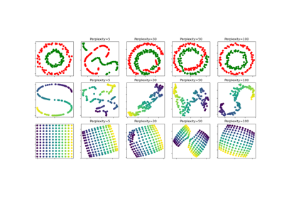
t-SNE: Der Effekt verschiedener Perplexitätswerte auf die Form

t-SNE: Der Effekt verschiedener Perplexitätswerte auf die Form

Vergleich von Manifold Learning Methoden

Vergleich von Manifold Learning Methoden

Annähernde nächste Nachbarn in TSNE

Annähernde nächste Nachbarn in TSNE

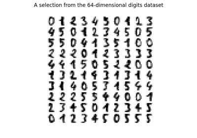
Manifold Learning auf handschriftlichen Ziffern: Locally Linear Embedding, Isomap…

Mannigfaltigkeitslernen auf handgeschriebenen Ziffern: Locally Linear Embedding, Isomap...