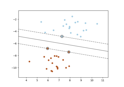
SVM: Trennende Hyperebene für unausgeglichene Klassen

Finden Sie die optimale trennende Hyperebene mit einem einfachen SVC für unausgeglichene Klassen.

Wir finden zunächst die trennende Ebene mit einem einfachen SVC und plotten dann (gestrichelt) die trennende Hyperebene mit automatischer Korrektur für unausgeglichene Klassen.

Hinweis

Dieses Beispiel funktioniert auch, wenn SVC(kernel="linear") durch SGDClassifier(loss="hinge") ersetzt wird. Wenn der Parameter loss des SGDClassifier auf hinge gesetzt wird, verhält er sich ähnlich wie ein SVC mit linearem Kernel.

Versuchen Sie zum Beispiel anstelle des SVC

clf = SGDClassifier(n_iter=100, alpha=0.01)

# Authors: The scikit-learn developers
# SPDX-License-Identifier: BSD-3-Clause

import matplotlib.lines as mlines
import matplotlib.pyplot as plt

from sklearn import svm
from sklearn.datasets import make_blobs
from sklearn.inspection import DecisionBoundaryDisplay

# we create two clusters of random points
n_samples_1 = 1000
n_samples_2 = 100
centers = [[0.0, 0.0], [2.0, 2.0]]
clusters_std = [1.5, 0.5]
X, y = make_blobs(
    n_samples=[n_samples_1, n_samples_2],
    centers=centers,
    cluster_std=clusters_std,
    random_state=0,
    shuffle=False,
)

# fit the model and get the separating hyperplane
clf = svm.SVC(kernel="linear", C=1.0)
clf.fit(X, y)

# fit the model and get the separating hyperplane using weighted classes
wclf = svm.SVC(kernel="linear", class_weight={1: 10})
wclf.fit(X, y)

# plot the samples
plt.scatter(X[:, 0], X[:, 1], c=y, cmap=plt.cm.Paired, edgecolors="k")

# plot the decision functions for both classifiers
ax = plt.gca()
disp = DecisionBoundaryDisplay.from_estimator(
    clf,
    X,
    plot_method="contour",
    colors="k",
    levels=[0],
    alpha=0.5,
    linestyles=["-"],
    ax=ax,
)

# plot decision boundary and margins for weighted classes
wdisp = DecisionBoundaryDisplay.from_estimator(
    wclf,
    X,
    plot_method="contour",
    colors="r",
    levels=[0],
    alpha=0.5,
    linestyles=["-"],
    ax=ax,
)

plt.legend(
    [
        mlines.Line2D([], [], color="k", label="non weighted"),
        mlines.Line2D([], [], color="r", label="weighted"),
    ],
    ["non weighted", "weighted"],
    loc="upper right",
)
plt.show()

Verwandte Beispiele

SVM: Maximum Margin Trennhyperplane

SVM: Maximum Margin Trennhyperplane

SGD: Maximum Margin Trennhyperplane

SGD: Maximum Margin Trennhyperplane

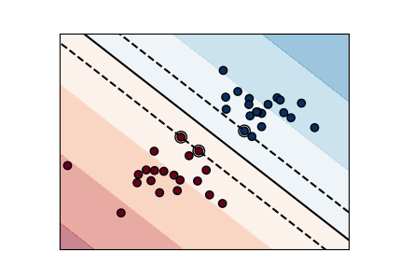
Verschiedene SVM-Klassifikatoren im Iris-Datensatz plotten

Verschiedene SVM-Klassifikatoren im Iris-Datensatz plotten

SVM-Randbeispiel

SVM-Randbeispiel