Hinweis
Zum Ende springen, um den vollständigen Beispielcode herunterzuladen oder dieses Beispiel in Ihrem Browser über JupyterLite oder Binder auszuführen.
Artenverbreitungsmodellierung#
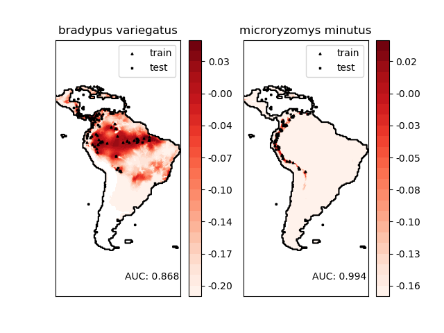
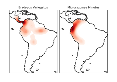
Die Modellierung der geografischen Verbreitung von Arten ist ein wichtiges Problem in der Naturschutzbiologie. In diesem Beispiel modellieren wir die geografische Verbreitung von zwei südamerikanischen Säugetieren anhand vergangener Beobachtungen und 14 Umweltvariablen. Da wir nur positive Beispiele haben (es gibt keine erfolglosen Beobachtungen), formulieren wir dieses Problem als Dichteschätzungsproblem und verwenden die OneClassSVM als unser Modellierungswerkzeug. Der Datensatz wird von Phillips et al. (2006) bereitgestellt. Falls verfügbar, verwendet das Beispiel basemap, um die Küstenlinien und Landesgrenzen Südamerikas zu zeichnen.
Die beiden Arten sind
Bradypus variegatus, das Braunkehlfaultier.
Microryzomys minutus, auch bekannt als kleiner Waldreisratte, ein Nagetier, das in Peru, Kolumbien, Ecuador, Peru und Venezuela lebt.
Referenzen#
„Maximum entropy modeling of species geographic distributions“ S. J. Phillips, R. P. Anderson, R. E. Schapire - Ecological Modelling, 190:231-259, 2006.
________________________________________________________________________________
Modeling distribution of species 'bradypus variegatus'
 - fit OneClassSVM ... done.
 - plot coastlines from coverage
 - predict species distribution

 Area under the ROC curve : 0.868443
________________________________________________________________________________
Modeling distribution of species 'microryzomys minutus'
 - fit OneClassSVM ... done.
 - plot coastlines from coverage
 - predict species distribution

 Area under the ROC curve : 0.993919

time elapsed: 7.26s
# Authors: The scikit-learn developers
# SPDX-License-Identifier: BSD-3-Clause

from time import time

import matplotlib.pyplot as plt
import numpy as np

from sklearn import metrics, svm
from sklearn.datasets import fetch_species_distributions
from sklearn.utils import Bunch

# if basemap is available, we'll use it.
# otherwise, we'll improvise later...
try:
    from mpl_toolkits.basemap import Basemap

    basemap = True
except ImportError:
    basemap = False


def construct_grids(batch):
    """Construct the map grid from the batch object

    Parameters
    ----------
    batch : Batch object
        The object returned by :func:`fetch_species_distributions`

    Returns
    -------
    (xgrid, ygrid) : 1-D arrays
        The grid corresponding to the values in batch.coverages
    """
    # x,y coordinates for corner cells
    xmin = batch.x_left_lower_corner + batch.grid_size
    xmax = xmin + (batch.Nx * batch.grid_size)
    ymin = batch.y_left_lower_corner + batch.grid_size
    ymax = ymin + (batch.Ny * batch.grid_size)

    # x coordinates of the grid cells
    xgrid = np.arange(xmin, xmax, batch.grid_size)
    # y coordinates of the grid cells
    ygrid = np.arange(ymin, ymax, batch.grid_size)

    return (xgrid, ygrid)


def create_species_bunch(species_name, train, test, coverages, xgrid, ygrid):
    """Create a bunch with information about a particular organism

    This will use the test/train record arrays to extract the
    data specific to the given species name.
    """
    bunch = Bunch(name=" ".join(species_name.split("_")[:2]))
    species_name = species_name.encode("ascii")
    points = dict(test=test, train=train)

    for label, pts in points.items():
        # choose points associated with the desired species
        pts = pts[pts["species"] == species_name]
        bunch["pts_%s" % label] = pts

        # determine coverage values for each of the training & testing points
        ix = np.searchsorted(xgrid, pts["dd long"])
        iy = np.searchsorted(ygrid, pts["dd lat"])
        bunch["cov_%s" % label] = coverages[:, -iy, ix].T

    return bunch


def plot_species_distribution(
    species=("bradypus_variegatus_0", "microryzomys_minutus_0"),
):
    """
    Plot the species distribution.
    """
    if len(species) > 2:
        print(
            "Note: when more than two species are provided,"
            " only the first two will be used"
        )

    t0 = time()

    # Load the compressed data
    data = fetch_species_distributions()

    # Set up the data grid
    xgrid, ygrid = construct_grids(data)

    # The grid in x,y coordinates
    X, Y = np.meshgrid(xgrid, ygrid[::-1])

    # create a bunch for each species
    BV_bunch = create_species_bunch(
        species[0], data.train, data.test, data.coverages, xgrid, ygrid
    )
    MM_bunch = create_species_bunch(
        species[1], data.train, data.test, data.coverages, xgrid, ygrid
    )

    # background points (grid coordinates) for evaluation
    np.random.seed(13)
    background_points = np.c_[
        np.random.randint(low=0, high=data.Ny, size=10000),
        np.random.randint(low=0, high=data.Nx, size=10000),
    ].T

    # We'll make use of the fact that coverages[6] has measurements at all
    # land points.  This will help us decide between land and water.
    land_reference = data.coverages[6]

    # Fit, predict, and plot for each species.
    for i, species in enumerate([BV_bunch, MM_bunch]):
        print("_" * 80)
        print("Modeling distribution of species '%s'" % species.name)

        # Standardize features
        mean = species.cov_train.mean(axis=0)
        std = species.cov_train.std(axis=0)
        train_cover_std = (species.cov_train - mean) / std

        # Fit OneClassSVM
        print(" - fit OneClassSVM ... ", end="")
        clf = svm.OneClassSVM(nu=0.1, kernel="rbf", gamma=0.5)
        clf.fit(train_cover_std)
        print("done.")

        # Plot map of South America
        plt.subplot(1, 2, i + 1)
        if basemap:
            print(" - plot coastlines using basemap")
            m = Basemap(
                projection="cyl",
                llcrnrlat=Y.min(),
                urcrnrlat=Y.max(),
                llcrnrlon=X.min(),
                urcrnrlon=X.max(),
                resolution="c",
            )
            m.drawcoastlines()
            m.drawcountries()
        else:
            print(" - plot coastlines from coverage")
            plt.contour(
                X, Y, land_reference, levels=[-9998], colors="k", linestyles="solid"
            )
            plt.xticks([])
            plt.yticks([])

        print(" - predict species distribution")

        # Predict species distribution using the training data
        Z = np.ones((data.Ny, data.Nx), dtype=np.float64)

        # We'll predict only for the land points.
        idx = (land_reference > -9999).nonzero()
        coverages_land = data.coverages[:, idx[0], idx[1]].T

        pred = clf.decision_function((coverages_land - mean) / std)
        Z *= pred.min()
        Z[idx[0], idx[1]] = pred

        levels = np.linspace(Z.min(), Z.max(), 25)
        Z[land_reference == -9999] = -9999

        # plot contours of the prediction
        plt.contourf(X, Y, Z, levels=levels, cmap=plt.cm.Reds)
        plt.colorbar(format="%.2f")

        # scatter training/testing points
        plt.scatter(
            species.pts_train["dd long"],
            species.pts_train["dd lat"],
            s=2**2,
            c="black",
            marker="^",
            label="train",
        )
        plt.scatter(
            species.pts_test["dd long"],
            species.pts_test["dd lat"],
            s=2**2,
            c="black",
            marker="x",
            label="test",
        )
        plt.legend()
        plt.title(species.name)
        plt.axis("equal")

        # Compute AUC with regards to background points
        pred_background = Z[background_points[0], background_points[1]]
        pred_test = clf.decision_function((species.cov_test - mean) / std)
        scores = np.r_[pred_test, pred_background]
        y = np.r_[np.ones(pred_test.shape), np.zeros(pred_background.shape)]
        fpr, tpr, thresholds = metrics.roc_curve(y, scores)
        roc_auc = metrics.auc(fpr, tpr)
        plt.text(-35, -70, "AUC: %.3f" % roc_auc, ha="right")
        print("\n Area under the ROC curve : %f" % roc_auc)

    print("\ntime elapsed: %.2fs" % (time() - t0))


plot_species_distribution()
plt.show()
Gesamtlaufzeit des Skripts: (0 Minuten 7,403 Sekunden)
Verwandte Beispiele
Testen der Signifikanz eines Klassifikations-Scores mit Permutationen