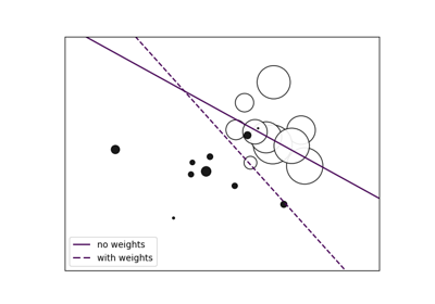
SVM: Gewichtete Stichproben

Zeichnet die Entscheidungsfunktion eines gewichteten Datensatzes, bei dem die Größe der Punkte proportional zu ihrem Gewicht ist.

Die Stichprobengewichtung skaliert den C-Parameter neu, was bedeutet, dass der Klassifikator mehr Wert darauf legt, diese Punkte korrekt zu klassifizieren. Der Effekt kann oft subtil sein. Um den Effekt hier zu betonen, erhöhen wir insbesondere das Gewicht der positiven Klasse, wodurch die Verformung der Entscheidungsgrenze sichtbarer wird.

# Authors: The scikit-learn developers
# SPDX-License-Identifier: BSD-3-Clause

import matplotlib.pyplot as plt
import numpy as np

from sklearn.datasets import make_classification
from sklearn.inspection import DecisionBoundaryDisplay
from sklearn.svm import SVC

X, y = make_classification(
    n_samples=1_000,
    n_features=2,
    n_informative=2,
    n_redundant=0,
    n_clusters_per_class=1,
    class_sep=1.1,
    weights=[0.9, 0.1],
    random_state=0,
)
# down-sample for plotting
rng = np.random.RandomState(0)
plot_indices = rng.choice(np.arange(X.shape[0]), size=100, replace=True)
X_plot, y_plot = X[plot_indices], y[plot_indices]


def plot_decision_function(classifier, sample_weight, axis, title):
    """Plot the synthetic data and the classifier decision function. Points with
    larger sample_weight are mapped to larger circles in the scatter plot."""
    axis.scatter(
        X_plot[:, 0],
        X_plot[:, 1],
        c=y_plot,
        s=100 * sample_weight[plot_indices],
        alpha=0.9,
        cmap=plt.cm.bone,
        edgecolors="black",
    )
    DecisionBoundaryDisplay.from_estimator(
        classifier,
        X_plot,
        response_method="decision_function",
        alpha=0.75,
        ax=axis,
        cmap=plt.cm.bone,
    )
    axis.axis("off")
    axis.set_title(title)


# we define constant weights as expected by the plotting function
sample_weight_constant = np.ones(len(X))
# assign random weights to all points
sample_weight_modified = abs(rng.randn(len(X)))
# assign bigger weights to the positive class
positive_class_indices = np.asarray(y == 1).nonzero()[0]
sample_weight_modified[positive_class_indices] *= 15

# This model does not include sample weights.
clf_no_weights = SVC(gamma=1)
clf_no_weights.fit(X, y)

# This other model includes sample weights.
clf_weights = SVC(gamma=1)
clf_weights.fit(X, y, sample_weight=sample_weight_modified)

fig, axes = plt.subplots(1, 2, figsize=(14, 6))
plot_decision_function(
    clf_no_weights, sample_weight_constant, axes[0], "Constant weights"
)
plot_decision_function(clf_weights, sample_weight_modified, axes[1], "Modified weights")

plt.show()

Verwandte Beispiele

Anpassen eines Elastic Net mit einer voreingestellten Gram-Matrix und gewichteten Stichproben

Anpassen eines Elastic Net mit einer voreingestellten Gram-Matrix und gewichteten Stichproben

SGD: Gewichtete Stichproben

SGD: Gewichtete Stichproben

Nearest Neighbors Regression

Nearest Neighbors Regression

Vergleich von linearen Bayes'schen Regressoren

Vergleich von linearen Bayes'schen Regressoren