Hinweis
Zum Ende springen, um den vollständigen Beispielcode herunterzuladen oder dieses Beispiel über JupyterLite oder Binder in Ihrem Browser auszuführen.
Restricted Boltzmann Machine Features für die Ziffernerkennung#
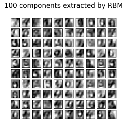
Für Graustufenbilddaten, bei denen Pixelwerte als Schwarzgrad auf weißem Hintergrund interpretiert werden können, wie bei der Erkennung handschriftlicher Ziffern, kann das Bernoulli Restricted Boltzmann Machine-Modell (BernoulliRBM) eine effektive nicht-lineare Merkmalsextraktion durchführen.
# Authors: The scikit-learn developers
# SPDX-License-Identifier: BSD-3-Clause
Daten generieren#
Um gute latente Darstellungen aus einem kleinen Datensatz zu lernen, generieren wir künstlich mehr beschriftete Daten, indem wir die Trainingsdaten mit linearen Verschiebungen von 1 Pixel in jede Richtung stören.
import numpy as np
from scipy.ndimage import convolve

from sklearn import datasets
from sklearn.model_selection import train_test_split
from sklearn.preprocessing import minmax_scale


def nudge_dataset(X, Y):
    """
    This produces a dataset 5 times bigger than the original one,
    by moving the 8x8 images in X around by 1px to left, right, down, up
    """
    direction_vectors = [
        [[0, 1, 0], [0, 0, 0], [0, 0, 0]],
        [[0, 0, 0], [1, 0, 0], [0, 0, 0]],
        [[0, 0, 0], [0, 0, 1], [0, 0, 0]],
        [[0, 0, 0], [0, 0, 0], [0, 1, 0]],
    ]

    def shift(x, w):
        return convolve(x.reshape((8, 8)), mode="constant", weights=w).ravel()

    X = np.concatenate(
        [X] + [np.apply_along_axis(shift, 1, X, vector) for vector in direction_vectors]
    )
    Y = np.concatenate([Y for _ in range(5)], axis=0)
    return X, Y


X, y = datasets.load_digits(return_X_y=True)
X = np.asarray(X, "float32")
X, Y = nudge_dataset(X, y)
X = minmax_scale(X, feature_range=(0, 1))  # 0-1 scaling

X_train, X_test, Y_train, Y_test = train_test_split(X, Y, test_size=0.2, random_state=0)
Modell Definition#
Wir erstellen eine Klassifizierungspipeline mit einem BernoulliRBM-Merkmalsextraktor und einem LogisticRegression-Klassifikator.
from sklearn import linear_model
from sklearn.neural_network import BernoulliRBM
from sklearn.pipeline import Pipeline

logistic = linear_model.LogisticRegression(solver="newton-cg", tol=1)
rbm = BernoulliRBM(random_state=0, verbose=True)

rbm_features_classifier = Pipeline(steps=[("rbm", rbm), ("logistic", logistic)])
Training#
Die Hyperparameter des gesamten Modells (Lernrate, Größe der versteckten Schicht, Regularisierung) wurden durch eine Grid-Suche optimiert, aber die Suche wird aus Laufzeitgründen hier nicht wiederholt.
from sklearn.base import clone

# Hyper-parameters. These were set by cross-validation,
# using a GridSearchCV. Here we are not performing cross-validation to
# save time.
rbm.learning_rate = 0.06
rbm.n_iter = 10

# More components tend to give better prediction performance, but larger
# fitting time
rbm.n_components = 100
logistic.C = 6000

# Training RBM-Logistic Pipeline
rbm_features_classifier.fit(X_train, Y_train)

# Training the Logistic regression classifier directly on the pixel
raw_pixel_classifier = clone(logistic)
raw_pixel_classifier.C = 100.0
raw_pixel_classifier.fit(X_train, Y_train)
[BernoulliRBM] Iteration 1, pseudo-likelihood = -25.57, time = 0.09s
[BernoulliRBM] Iteration 2, pseudo-likelihood = -23.68, time = 0.13s
[BernoulliRBM] Iteration 3, pseudo-likelihood = -22.88, time = 0.13s
[BernoulliRBM] Iteration 4, pseudo-likelihood = -21.91, time = 0.12s
[BernoulliRBM] Iteration 5, pseudo-likelihood = -21.79, time = 0.12s
[BernoulliRBM] Iteration 6, pseudo-likelihood = -20.96, time = 0.12s
[BernoulliRBM] Iteration 7, pseudo-likelihood = -20.88, time = 0.12s
[BernoulliRBM] Iteration 8, pseudo-likelihood = -20.50, time = 0.12s
[BernoulliRBM] Iteration 9, pseudo-likelihood = -20.34, time = 0.12s
[BernoulliRBM] Iteration 10, pseudo-likelihood = -20.21, time = 0.12s
Bewertung#
from sklearn import metrics

Y_pred = rbm_features_classifier.predict(X_test)
print(
    "Logistic regression using RBM features:\n%s\n"
    % (metrics.classification_report(Y_test, Y_pred))
)
/home/circleci/project/sklearn/metrics/_classification.py:1833: UndefinedMetricWarning:

Precision is ill-defined and being set to 0.0 in labels with no predicted samples. Use `zero_division` parameter to control this behavior.

/home/circleci/project/sklearn/metrics/_classification.py:1833: UndefinedMetricWarning:

Precision is ill-defined and being set to 0.0 in labels with no predicted samples. Use `zero_division` parameter to control this behavior.

/home/circleci/project/sklearn/metrics/_classification.py:1833: UndefinedMetricWarning:

Precision is ill-defined and being set to 0.0 in labels with no predicted samples. Use `zero_division` parameter to control this behavior.

Logistic regression using RBM features:
              precision    recall  f1-score   support

           0       0.10      1.00      0.18       174
           1       0.00      0.00      0.00       184
           2       0.00      0.00      0.00       166
           3       0.00      0.00      0.00       194
           4       0.00      0.00      0.00       186
           5       0.00      0.00      0.00       181
           6       0.00      0.00      0.00       207
           7       0.00      0.00      0.00       154
           8       0.00      0.00      0.00       182
           9       0.00      0.00      0.00       169

    accuracy                           0.10      1797
   macro avg       0.01      0.10      0.02      1797
weighted avg       0.01      0.10      0.02      1797
Y_pred = raw_pixel_classifier.predict(X_test)
print(
    "Logistic regression using raw pixel features:\n%s\n"
    % (metrics.classification_report(Y_test, Y_pred))
)
/home/circleci/project/sklearn/metrics/_classification.py:1833: UndefinedMetricWarning:

Precision is ill-defined and being set to 0.0 in labels with no predicted samples. Use `zero_division` parameter to control this behavior.

/home/circleci/project/sklearn/metrics/_classification.py:1833: UndefinedMetricWarning:

Precision is ill-defined and being set to 0.0 in labels with no predicted samples. Use `zero_division` parameter to control this behavior.

/home/circleci/project/sklearn/metrics/_classification.py:1833: UndefinedMetricWarning:

Precision is ill-defined and being set to 0.0 in labels with no predicted samples. Use `zero_division` parameter to control this behavior.

Logistic regression using raw pixel features:
              precision    recall  f1-score   support

           0       0.10      1.00      0.18       174
           1       0.00      0.00      0.00       184
           2       0.00      0.00      0.00       166
           3       0.00      0.00      0.00       194
           4       0.00      0.00      0.00       186
           5       0.00      0.00      0.00       181
           6       0.00      0.00      0.00       207
           7       0.00      0.00      0.00       154
           8       0.00      0.00      0.00       182
           9       0.00      0.00      0.00       169

    accuracy                           0.10      1797
   macro avg       0.01      0.10      0.02      1797
weighted avg       0.01      0.10      0.02      1797
Die von der BernoulliRBM extrahierten Merkmale helfen, die Klassifikationsgenauigkeit im Vergleich zur logistischen Regression auf Rohpixeln zu verbessern.
Plotten#
import matplotlib.pyplot as plt

plt.figure(figsize=(4.2, 4))
for i, comp in enumerate(rbm.components_):
    plt.subplot(10, 10, i + 1)
    plt.imshow(comp.reshape((8, 8)), cmap=plt.cm.gray_r, interpolation="nearest")
    plt.xticks(())
    plt.yticks(())
plt.suptitle("100 components extracted by RBM", fontsize=16)
plt.subplots_adjust(0.08, 0.02, 0.92, 0.85, 0.08, 0.23)

plt.show()
Gesamtlaufzeit des Skripts: (0 Minuten 2,139 Sekunden)
Verwandte Beispiele
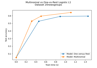
Multiklassen-Sparse-Logistische-Regression auf 20newgroups
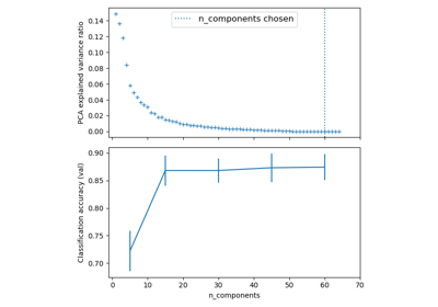
Pipelining: Verkettung einer PCA und einer logistischen Regression
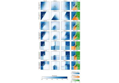
Entscheidungsgrenzen von multinomialer und One-vs-Rest Logistischer Regression