Auswahl der Anzahl von Clustern mit Silhouettenanalyse bei KMeans-Clustering

Die Silhouettenanalyse kann verwendet werden, um den Trennungsabstand zwischen den resultierenden Clustern zu untersuchen. Das Silhouetten-Diagramm zeigt ein Maß dafür, wie nah jeder Punkt in einem Cluster an Punkten in benachbarten Clustern ist, und bietet somit eine Möglichkeit, Parameter wie die Anzahl der Cluster visuell zu bewerten. Dieses Maß reicht von [-1, 1].

Silhouettenkoeffizienten (wie diese Werte bezeichnet werden) nahe +1 deuten darauf hin, dass sich die Stichprobe weit von den benachbarten Clustern entfernt befindet. Ein Wert von 0 deutet darauf hin, dass sich die Stichprobe an oder sehr nahe an der Entscheidungsgrenze zwischen zwei benachbarten Clustern befindet, und negative Werte deuten darauf hin, dass diese Stichproben möglicherweise dem falschen Cluster zugeordnet wurden.

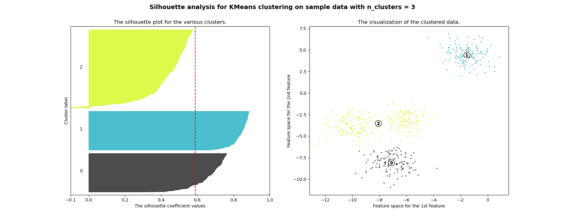
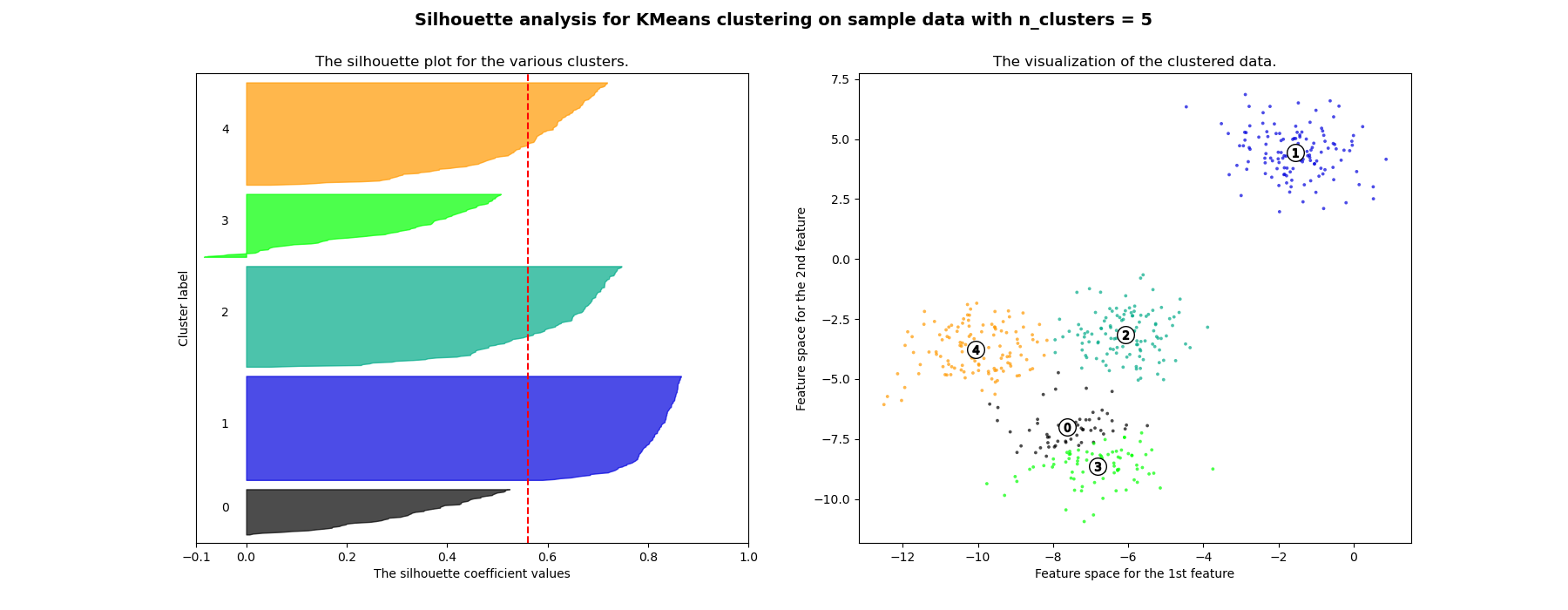
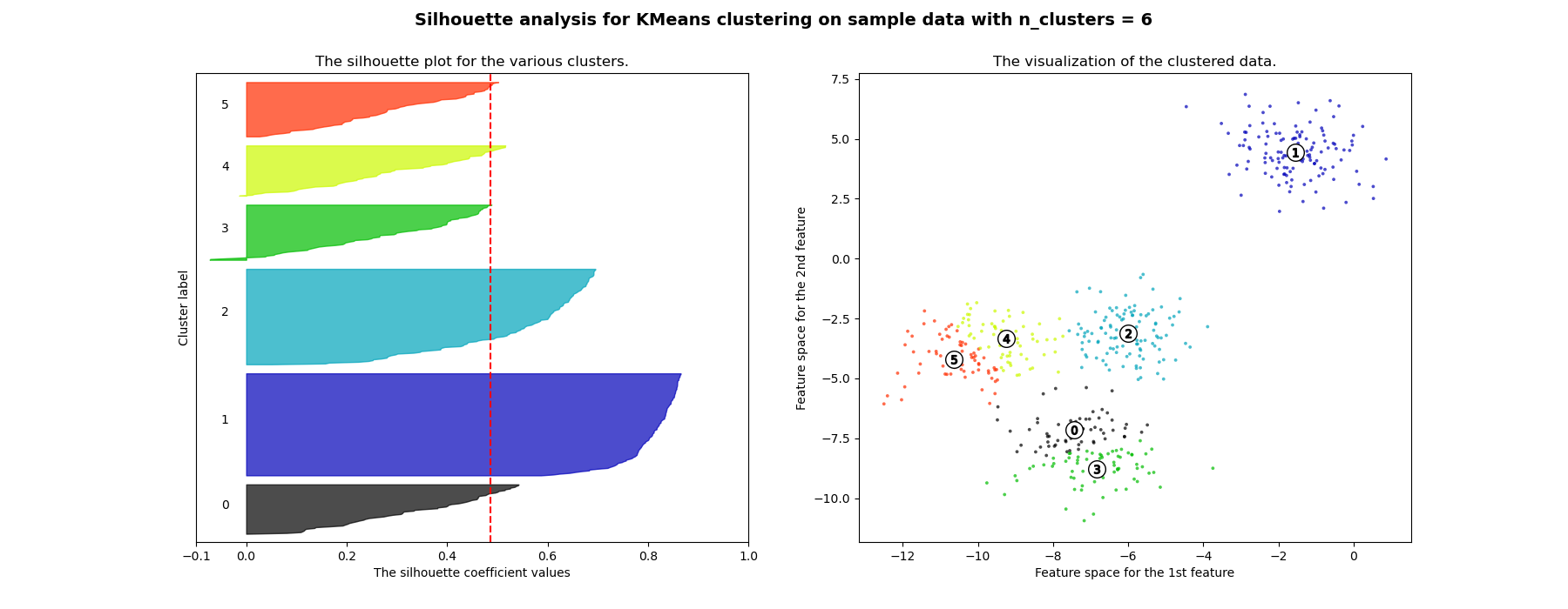
In diesem Beispiel wird die Silhouettenanalyse verwendet, um einen optimalen Wert für n_clusters zu wählen. Das Silhouetten-Diagramm zeigt, dass die n_clusters-Werte von 3, 5 und 6 eine schlechte Wahl für die gegebenen Daten sind, da Cluster mit unterdurchschnittlichen Silhouetten-Scores und auch aufgrund großer Schwankungen in der Größe der Silhouetten-Diagramme vorhanden sind. Die Silhouettenanalyse ist bei der Entscheidung zwischen 2 und 4 ambivalenter.

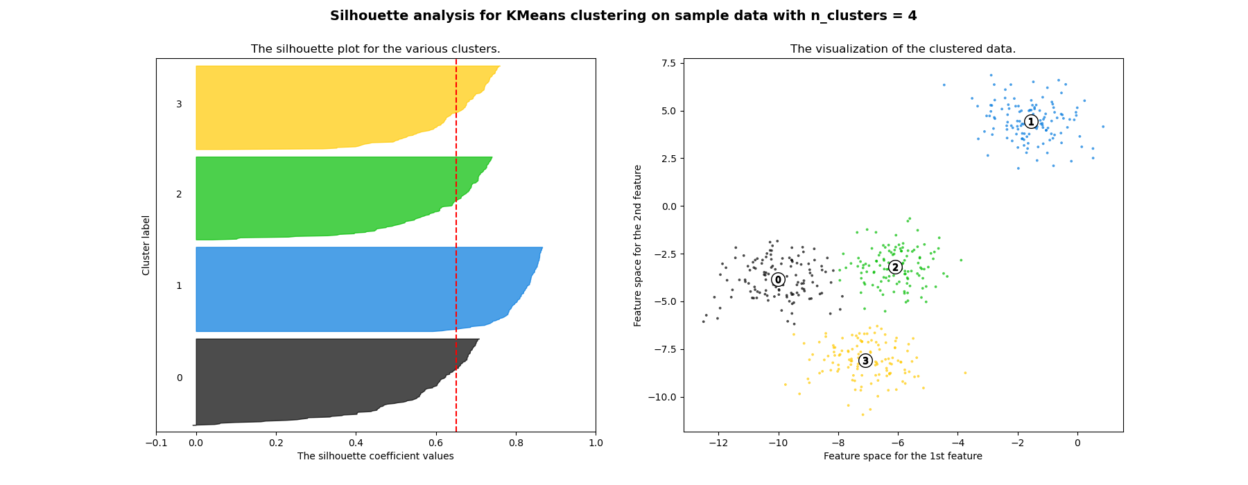
Auch aus der Dicke des Silhouetten-Diagramms kann die Clustergröße visualisiert werden. Das Silhouetten-Diagramm für Cluster 0, wenn n_clusters gleich 2 ist, ist aufgrund der Gruppierung der 3 Untercluster zu einem großen Cluster größer. Wenn jedoch n_clusters gleich 4 ist, sind alle Diagramme mehr oder weniger gleich dick und somit von ähnlicher Größe, was auch aus dem beschrifteten Streudiagramm auf der rechten Seite ersichtlich ist.

• 
• 
• 
• 
• 

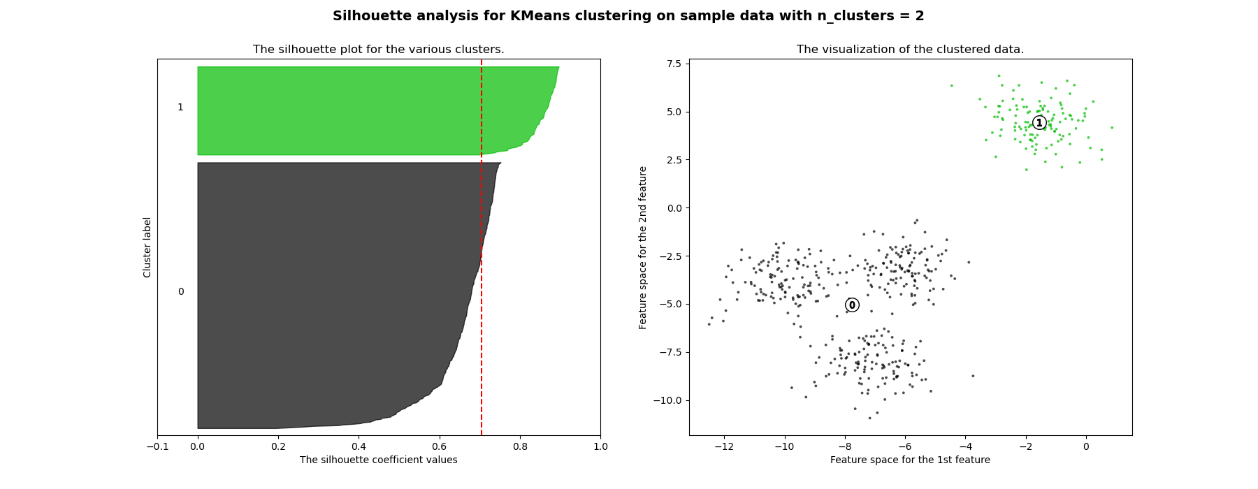
For n_clusters = 2 The average silhouette_score is : 0.7049787496083262
For n_clusters = 3 The average silhouette_score is : 0.5882004012129721
For n_clusters = 4 The average silhouette_score is : 0.6505186632729437
For n_clusters = 5 The average silhouette_score is : 0.561464362648773
For n_clusters = 6 The average silhouette_score is : 0.4857596147013469

# Authors: The scikit-learn developers
# SPDX-License-Identifier: BSD-3-Clause

import matplotlib.cm as cm
import matplotlib.pyplot as plt
import numpy as np

from sklearn.cluster import KMeans
from sklearn.datasets import make_blobs
from sklearn.metrics import silhouette_samples, silhouette_score

# Generating the sample data from make_blobs
# This particular setting has one distinct cluster and 3 clusters placed close
# together.
X, y = make_blobs(
    n_samples=500,
    n_features=2,
    centers=4,
    cluster_std=1,
    center_box=(-10.0, 10.0),
    shuffle=True,
    random_state=1,
)  # For reproducibility

range_n_clusters = [2, 3, 4, 5, 6]

for n_clusters in range_n_clusters:
    # Create a subplot with 1 row and 2 columns
    fig, (ax1, ax2) = plt.subplots(1, 2)
    fig.set_size_inches(18, 7)

    # The 1st subplot is the silhouette plot
    # The silhouette coefficient can range from -1, 1 but in this example all
    # lie within [-0.1, 1]
    ax1.set_xlim([-0.1, 1])
    # The (n_clusters+1)*10 is for inserting blank space between silhouette
    # plots of individual clusters, to demarcate them clearly.
    ax1.set_ylim([0, len(X) + (n_clusters + 1) * 10])

    # Initialize the clusterer with n_clusters value and a random generator
    # seed of 10 for reproducibility.
    clusterer = KMeans(n_clusters=n_clusters, random_state=10)
    cluster_labels = clusterer.fit_predict(X)

    # The silhouette_score gives the average value for all the samples.
    # This gives a perspective into the density and separation of the formed
    # clusters
    silhouette_avg = silhouette_score(X, cluster_labels)
    print(
        "For n_clusters =",
        n_clusters,
        "The average silhouette_score is :",
        silhouette_avg,
    )

    # Compute the silhouette scores for each sample
    sample_silhouette_values = silhouette_samples(X, cluster_labels)

    y_lower = 10
    for i in range(n_clusters):
        # Aggregate the silhouette scores for samples belonging to
        # cluster i, and sort them
        ith_cluster_silhouette_values = sample_silhouette_values[cluster_labels == i]

        ith_cluster_silhouette_values.sort()

        size_cluster_i = ith_cluster_silhouette_values.shape[0]
        y_upper = y_lower + size_cluster_i

        color = cm.nipy_spectral(float(i) / n_clusters)
        ax1.fill_betweenx(
            np.arange(y_lower, y_upper),
            0,
            ith_cluster_silhouette_values,
            facecolor=color,
            edgecolor=color,
            alpha=0.7,
        )

        # Label the silhouette plots with their cluster numbers at the middle
        ax1.text(-0.05, y_lower + 0.5 * size_cluster_i, str(i))

        # Compute the new y_lower for next plot
        y_lower = y_upper + 10  # 10 for the 0 samples

    ax1.set_title("The silhouette plot for the various clusters.")
    ax1.set_xlabel("The silhouette coefficient values")
    ax1.set_ylabel("Cluster label")

    # The vertical line for average silhouette score of all the values
    ax1.axvline(x=silhouette_avg, color="red", linestyle="--")

    ax1.set_yticks([])  # Clear the yaxis labels / ticks
    ax1.set_xticks([-0.1, 0, 0.2, 0.4, 0.6, 0.8, 1])

    # 2nd Plot showing the actual clusters formed
    colors = cm.nipy_spectral(cluster_labels.astype(float) / n_clusters)
    ax2.scatter(
        X[:, 0], X[:, 1], marker=".", s=30, lw=0, alpha=0.7, c=colors, edgecolor="k"
    )

    # Labeling the clusters
    centers = clusterer.cluster_centers_
    # Draw white circles at cluster centers
    ax2.scatter(
        centers[:, 0],
        centers[:, 1],
        marker="o",
        c="white",
        alpha=1,
        s=200,
        edgecolor="k",
    )

    for i, c in enumerate(centers):
        ax2.scatter(c[0], c[1], marker="$%d$" % i, alpha=1, s=50, edgecolor="k")

    ax2.set_title("The visualization of the clustered data.")
    ax2.set_xlabel("Feature space for the 1st feature")
    ax2.set_ylabel("Feature space for the 2nd feature")

    plt.suptitle(
        "Silhouette analysis for KMeans clustering on sample data with n_clusters = %d"
        % n_clusters,
        fontsize=14,
        fontweight="bold",
    )

plt.show()

Verwandte Beispiele

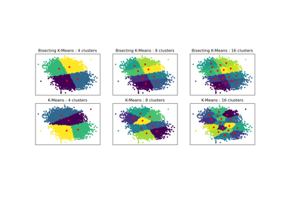
Vergleich der Leistung von Bisecting K-Means und Regular K-Means

Vergleich der Leistung von Bisecting K-Means und Regular K-Means

Demo des DBSCAN Clustering Algorithmus

Demo des DBSCAN Clustering Algorithmus

Clustering von Textdokumenten mit K-Means

Clustering von Textdokumenten mit K-Means

Agglomeratives Clustering mit verschiedenen Metriken

Agglomeratives Clustering mit verschiedenen Metriken