Hinweis
Zum Ende springen, um den vollständigen Beispielcode herunterzuladen oder dieses Beispiel über JupyterLite oder Binder in Ihrem Browser auszuführen.
Lasso, Lasso-LARS und Elastic Net Pfade#
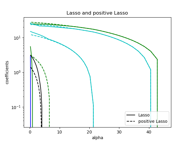
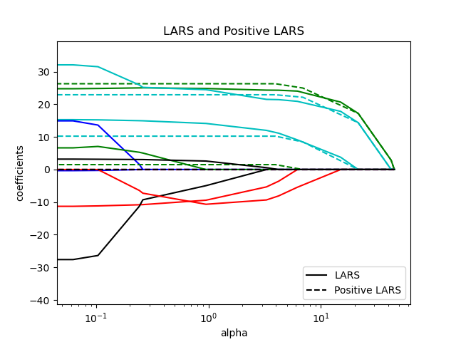
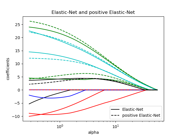
Dieses Beispiel zeigt, wie die „Pfade“ von Koeffizienten entlang der Lasso-, Lasso-LARS- und Elastic Net-Regularisierungspfade berechnet werden. Mit anderen Worten, es zeigt die Beziehung zwischen dem Regularisierungsparameter (alpha) und den Koeffizienten.
Lasso und Lasso-LARS erzwingen eine Sparsity-Beschränkung auf die Koeffizienten, was dazu führt, dass einige von ihnen null werden. Elastic Net ist eine Verallgemeinerung von Lasso, die einen L2-Strafterm zum L1-Strafterm hinzufügt. Dies ermöglicht, dass einige Koeffizienten nicht null sind, während gleichzeitig Sparsity gefördert wird.
Lasso und Elastic Net verwenden eine Koordinatensenkungsmethode zur Berechnung der Pfade, während Lasso-LARS den LARS-Algorithmus zur Berechnung der Pfade verwendet.
Die Pfade werden mit lasso_path, lars_path und enet_path berechnet.
Die Ergebnisse zeigen verschiedene Vergleichsdiagramme
Vergleich von Lasso und Lasso-LARS
Vergleich von Lasso und Elastic Net
Vergleich von Lasso mit positivem Lasso
Vergleich von LARS und positivem LARS
Vergleich von Elastic Net und positivem Elastic Net
Jedes Diagramm zeigt, wie sich die Modellkoeffizienten mit der Änderung der Regularisierungsstärke ändern, und bietet Einblicke in das Verhalten dieser Modelle unter verschiedenen Beschränkungen.


Computing regularization path using the lasso...
Computing regularization path using the positive lasso...
Computing regularization path using the LARS...
Computing regularization path using the positive LARS...
Computing regularization path using the elastic net...
Computing regularization path using the positive elastic net...
# Authors: The scikit-learn developers
# SPDX-License-Identifier: BSD-3-Clause

from itertools import cycle

import matplotlib.pyplot as plt

from sklearn.datasets import load_diabetes
from sklearn.linear_model import enet_path, lars_path, lasso_path

X, y = load_diabetes(return_X_y=True)
X /= X.std(axis=0)  # Standardize data (easier to set the l1_ratio parameter)

# Compute paths

eps = 5e-3  # the smaller it is the longer is the path

print("Computing regularization path using the lasso...")
alphas_lasso, coefs_lasso, _ = lasso_path(X, y, eps=eps)

print("Computing regularization path using the positive lasso...")
alphas_positive_lasso, coefs_positive_lasso, _ = lasso_path(
    X, y, eps=eps, positive=True
)

print("Computing regularization path using the LARS...")
alphas_lars, _, coefs_lars = lars_path(X, y, method="lasso")

print("Computing regularization path using the positive LARS...")
alphas_positive_lars, _, coefs_positive_lars = lars_path(
    X, y, method="lasso", positive=True
)

print("Computing regularization path using the elastic net...")
alphas_enet, coefs_enet, _ = enet_path(X, y, eps=eps, l1_ratio=0.8)

print("Computing regularization path using the positive elastic net...")
alphas_positive_enet, coefs_positive_enet, _ = enet_path(
    X, y, eps=eps, l1_ratio=0.8, positive=True
)

# Display results

plt.figure(1)
colors = cycle(["b", "r", "g", "c", "k"])
for coef_lasso, coef_lars, c in zip(coefs_lasso, coefs_lars, colors):
    l1 = plt.semilogx(alphas_lasso, coef_lasso, c=c)
    l2 = plt.semilogx(alphas_lars, coef_lars, linestyle="--", c=c)

plt.xlabel("alpha")
plt.ylabel("coefficients")
plt.title("Lasso and LARS Paths")
plt.legend((l1[-1], l2[-1]), ("Lasso", "LARS"), loc="lower right")
plt.axis("tight")

plt.figure(2)
colors = cycle(["b", "r", "g", "c", "k"])
for coef_l, coef_e, c in zip(coefs_lasso, coefs_enet, colors):
    l1 = plt.semilogx(alphas_lasso, coef_l, c=c)
    l2 = plt.semilogx(alphas_enet, coef_e, linestyle="--", c=c)

plt.xlabel("alpha")
plt.ylabel("coefficients")
plt.title("Lasso and Elastic-Net Paths")
plt.legend((l1[-1], l2[-1]), ("Lasso", "Elastic-Net"), loc="lower right")
plt.axis("tight")


plt.figure(3)
for coef_l, coef_pl, c in zip(coefs_lasso, coefs_positive_lasso, colors):
    l1 = plt.semilogy(alphas_lasso, coef_l, c=c)
    l2 = plt.semilogy(alphas_positive_lasso, coef_pl, linestyle="--", c=c)

plt.xlabel("alpha")
plt.ylabel("coefficients")
plt.title("Lasso and positive Lasso")
plt.legend((l1[-1], l2[-1]), ("Lasso", "positive Lasso"), loc="lower right")
plt.axis("tight")


plt.figure(4)
colors = cycle(["b", "r", "g", "c", "k"])
for coef_lars, coef_positive_lars, c in zip(coefs_lars, coefs_positive_lars, colors):
    l1 = plt.semilogx(alphas_lars, coef_lars, c=c)
    l2 = plt.semilogx(alphas_positive_lars, coef_positive_lars, linestyle="--", c=c)

plt.xlabel("alpha")
plt.ylabel("coefficients")
plt.title("LARS and Positive LARS")
plt.legend((l1[-1], l2[-1]), ("LARS", "Positive LARS"), loc="lower right")
plt.axis("tight")

plt.figure(5)
for coef_e, coef_pe, c in zip(coefs_enet, coefs_positive_enet, colors):
    l1 = plt.semilogx(alphas_enet, coef_e, c=c)
    l2 = plt.semilogx(alphas_positive_enet, coef_pe, linestyle="--", c=c)

plt.xlabel("alpha")
plt.ylabel("coefficients")
plt.title("Elastic-Net and positive Elastic-Net")
plt.legend((l1[-1], l2[-1]), ("Elastic-Net", "positive Elastic-Net"), loc="lower right")
plt.axis("tight")
plt.show()
Gesamtlaufzeit des Skripts: (0 Minuten 0,844 Sekunden)
Verwandte Beispiele