Feature Agglomeration vs. univariate Auswahl

Dieses Beispiel vergleicht 2 Strategien zur Dimensionsreduktion

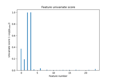
• univariate Merkmalsauswahl mit Anova

• Feature Agglomeration mit Ward hierarchischem Clustering

Beide Methoden werden in einem Regressionsproblem mit einem BayesianRidge als überwachtem Schätzer verglichen.

# Authors: The scikit-learn developers
# SPDX-License-Identifier: BSD-3-Clause

import shutil
import tempfile

import matplotlib.pyplot as plt
import numpy as np
from joblib import Memory
from scipy import linalg, ndimage

from sklearn import feature_selection
from sklearn.cluster import FeatureAgglomeration
from sklearn.feature_extraction.image import grid_to_graph
from sklearn.linear_model import BayesianRidge
from sklearn.model_selection import GridSearchCV, KFold
from sklearn.pipeline import Pipeline

Parameter setzen

n_samples = 200
size = 40  # image size
roi_size = 15
snr = 5.0
np.random.seed(0)

Daten generieren

coef = np.zeros((size, size))
coef[0:roi_size, 0:roi_size] = -1.0
coef[-roi_size:, -roi_size:] = 1.0

X = np.random.randn(n_samples, size**2)
for x in X:  # smooth data
    x[:] = ndimage.gaussian_filter(x.reshape(size, size), sigma=1.0).ravel()
X -= X.mean(axis=0)
X /= X.std(axis=0)

y = np.dot(X, coef.ravel())

Rauschen hinzufügen

noise = np.random.randn(y.shape[0])
noise_coef = (linalg.norm(y, 2) / np.exp(snr / 20.0)) / linalg.norm(noise, 2)
y += noise_coef * noise

Koeffizienten eines Bayesian Ridge mit GridSearch berechnen

cv = KFold(2)  # cross-validation generator for model selection
ridge = BayesianRidge()
cachedir = tempfile.mkdtemp()
mem = Memory(location=cachedir, verbose=1)

Ward Agglomeration gefolgt von BayesianRidge

connectivity = grid_to_graph(n_x=size, n_y=size)
ward = FeatureAgglomeration(n_clusters=10, connectivity=connectivity, memory=mem)
clf = Pipeline([("ward", ward), ("ridge", ridge)])
# Select the optimal number of parcels with grid search
clf = GridSearchCV(clf, {"ward__n_clusters": [10, 20, 30]}, n_jobs=1, cv=cv)
clf.fit(X, y)  # set the best parameters
coef_ = clf.best_estimator_.steps[-1][1].coef_
coef_ = clf.best_estimator_.steps[0][1].inverse_transform(coef_)
coef_agglomeration_ = coef_.reshape(size, size)

________________________________________________________________________________
[Memory] Calling sklearn.cluster._agglomerative.ward_tree...
ward_tree(array([[-0.451933, ..., -0.675318],
       ...,
       [ 0.275706, ..., -1.085711]], shape=(1600, 100)), connectivity=<COOrdinate sparse matrix of dtype 'int64'
        with 7840 stored elements and shape (1600, 1600)>, n_clusters=None, return_distance=False)
________________________________________________________ward_tree - 0.0s, 0.0min
________________________________________________________________________________
[Memory] Calling sklearn.cluster._agglomerative.ward_tree...
ward_tree(array([[ 0.905206, ...,  0.161245],
       ...,
       [-0.849835, ..., -1.091621]], shape=(1600, 100)), connectivity=<COOrdinate sparse matrix of dtype 'int64'
        with 7840 stored elements and shape (1600, 1600)>, n_clusters=None, return_distance=False)
________________________________________________________ward_tree - 0.0s, 0.0min
________________________________________________________________________________
[Memory] Calling sklearn.cluster._agglomerative.ward_tree...
ward_tree(array([[ 0.905206, ..., -0.675318],
       ...,
       [-0.849835, ..., -1.085711]], shape=(1600, 200)), connectivity=<COOrdinate sparse matrix of dtype 'int64'
        with 7840 stored elements and shape (1600, 1600)>, n_clusters=None, return_distance=False)
________________________________________________________ward_tree - 0.0s, 0.0min

Anova univariate Merkmalsauswahl gefolgt von BayesianRidge

f_regression = mem.cache(feature_selection.f_regression)  # caching function
anova = feature_selection.SelectPercentile(f_regression)
clf = Pipeline([("anova", anova), ("ridge", ridge)])
# Select the optimal percentage of features with grid search
clf = GridSearchCV(clf, {"anova__percentile": [5, 10, 20]}, cv=cv)
clf.fit(X, y)  # set the best parameters
coef_ = clf.best_estimator_.steps[-1][1].coef_
coef_ = clf.best_estimator_.steps[0][1].inverse_transform(coef_.reshape(1, -1))
coef_selection_ = coef_.reshape(size, size)

________________________________________________________________________________
[Memory] Calling sklearn.feature_selection._univariate_selection.f_regression...
f_regression(array([[-0.451933, ...,  0.275706],
       ...,
       [-0.675318, ..., -1.085711]], shape=(100, 1600)),
array([ 25.267703, ..., -25.026711], shape=(100,)))
_____________________________________________________f_regression - 0.0s, 0.0min
________________________________________________________________________________
[Memory] Calling sklearn.feature_selection._univariate_selection.f_regression...
f_regression(array([[ 0.905206, ..., -0.849835],
       ...,
       [ 0.161245, ..., -1.091621]], shape=(100, 1600)),
array([ -27.447268, ..., -112.638768], shape=(100,)))
_____________________________________________________f_regression - 0.0s, 0.0min
________________________________________________________________________________
[Memory] Calling sklearn.feature_selection._univariate_selection.f_regression...
f_regression(array([[ 0.905206, ..., -0.849835],
       ...,
       [-0.675318, ..., -1.085711]], shape=(200, 1600)),
array([-27.447268, ..., -25.026711], shape=(200,)))
_____________________________________________________f_regression - 0.0s, 0.0min

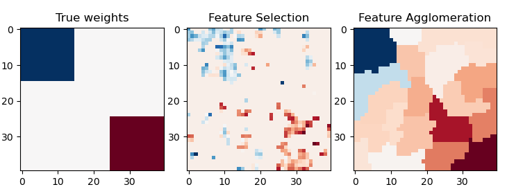
Invertieren der Transformation, um die Ergebnisse auf einem Bild darzustellen

plt.close("all")
plt.figure(figsize=(7.3, 2.7))
plt.subplot(1, 3, 1)
plt.imshow(coef, interpolation="nearest", cmap=plt.cm.RdBu_r)
plt.title("True weights")
plt.subplot(1, 3, 2)
plt.imshow(coef_selection_, interpolation="nearest", cmap=plt.cm.RdBu_r)
plt.title("Feature Selection")
plt.subplot(1, 3, 3)
plt.imshow(coef_agglomeration_, interpolation="nearest", cmap=plt.cm.RdBu_r)
plt.title("Feature Agglomeration")
plt.subplots_adjust(0.04, 0.0, 0.98, 0.94, 0.16, 0.26)
plt.show()

Versuch, das temporäre Verzeichnis zu entfernen, aber keine Sorge, wenn es fehlschlägt

shutil.rmtree(cachedir, ignore_errors=True)

Verwandte Beispiele

Eine Demo des strukturierten Ward Hierarchischen Clusterings auf einem Bild von Münzen

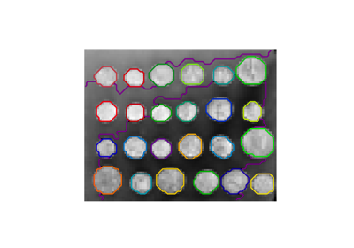
Eine Demo des strukturierten Ward Hierarchischen Clusterings auf einem Bild von Münzen

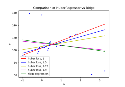
HuberRegressor vs Ridge auf Datensatz mit starken Ausreißern

HuberRegressor vs Ridge auf Datensatz mit starken Ausreißern

Univariate Merkmalsauswahl

Univariate Merkmalsauswahl

Orthogonal Matching Pursuit

Orthogonal Matching Pursuit