Hinweis
Zum Ende springen, um den vollständigen Beispielcode herunterzuladen oder dieses Beispiel über JupyterLite oder Binder in Ihrem Browser auszuführen.
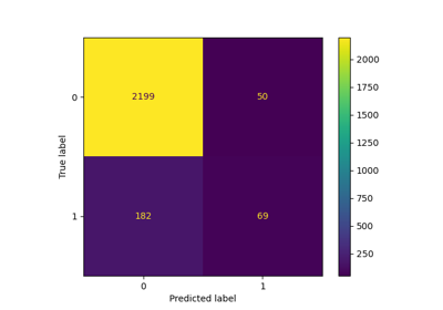
Leistungsbewertung eines Klassifikators mit einer Konfusionsmatrix#
Beispiel für die Verwendung einer Konfusionsmatrix zur Bewertung der Qualität der Ausgabe eines Klassifikators auf dem Iris-Datensatz. Die Diagonalelemente stellen die Anzahl der Punkte dar, bei denen das vorhergesagte Label mit dem tatsächlichen Label übereinstimmt, während die Nicht-Diagonalelemente diejenigen sind, die vom Klassifikator falsch zugeordnet wurden. Je höher die Diagonalwerte der Konfusionsmatrix, desto besser, was viele korrekte Vorhersagen anzeigt.
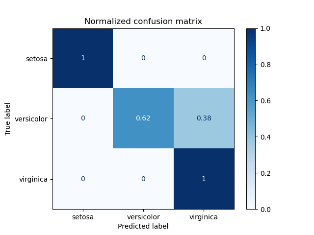
Die Abbildungen zeigen die Konfusionsmatrix mit und ohne Normalisierung nach der Klassengröße (Anzahl der Elemente in jeder Klasse). Diese Art der Normalisierung kann bei Klassenungleichgewichten interessant sein, um eine visuellere Interpretation zu erhalten, welche Klasse falsch klassifiziert wird.
Hier sind die Ergebnisse nicht so gut, wie sie sein könnten, da unsere Wahl des Regularisierungsparameters C nicht die beste war. In realen Anwendungen wird dieser Parameter normalerweise mit Anpassen der Hyperparameter eines Schätzers ausgewählt.
# Authors: The scikit-learn developers
# SPDX-License-Identifier: BSD-3-Clause

import matplotlib.pyplot as plt
import numpy as np

from sklearn import datasets, svm
from sklearn.metrics import ConfusionMatrixDisplay
from sklearn.model_selection import train_test_split

# import some data to play with
iris = datasets.load_iris()
X = iris.data
y = iris.target
class_names = iris.target_names

# Split the data into a training set and a test set
X_train, X_test, y_train, y_test = train_test_split(X, y, random_state=0)

# Run classifier, using a model that is too regularized (C too low) to see
# the impact on the results
classifier = svm.SVC(kernel="linear", C=0.01).fit(X_train, y_train)

np.set_printoptions(precision=2)

# Plot non-normalized confusion matrix
titles_options = [
    ("Confusion matrix, without normalization", None),
    ("Normalized confusion matrix", "true"),
]
for title, normalize in titles_options:
    disp = ConfusionMatrixDisplay.from_estimator(
        classifier,
        X_test,
        y_test,
        display_labels=class_names,
        cmap=plt.cm.Blues,
        normalize=normalize,
    )
    disp.ax_.set_title(title)

    print(title)
    print(disp.confusion_matrix)

plt.show()
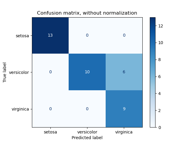
Confusion matrix, without normalization
[[13  0  0]
 [ 0 10  6]
 [ 0  0  9]]
Normalized confusion matrix
[[1.   0.   0.  ]
 [0.   0.62 0.38]
 [0.   0.   1.  ]]
Binäre Klassifizierung#
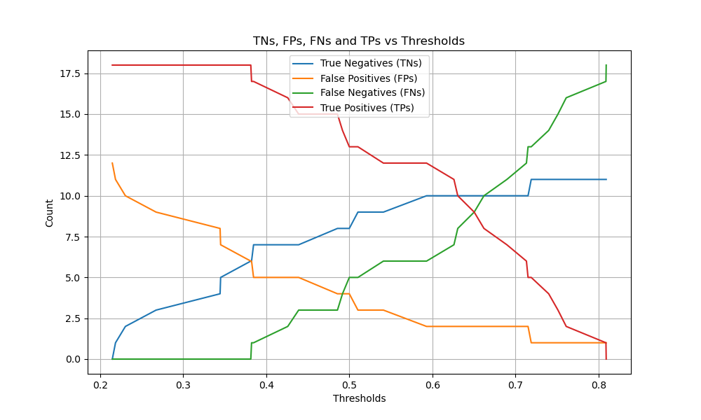
Für binäre Probleme verfügt sklearn.metrics.confusion_matrix über die ravel-Methode, die wir verwenden können, um die Anzahl von True Negatives, False Positives, False Negatives und True Positives zu erhalten.
Um die Anzahlen von True Negatives, False Positives, False Negatives und True Positives bei verschiedenen Schwellenwerten zu erhalten, kann man sklearn.metrics.confusion_matrix_at_thresholds verwenden. Dies ist grundlegend für binäre Klassifizierungsmetriken wie roc_auc_score und det_curve.
from sklearn.datasets import make_classification
from sklearn.metrics import confusion_matrix_at_thresholds

X, y = make_classification(
    n_samples=100,
    n_features=20,
    n_informative=20,
    n_redundant=0,
    n_classes=2,
    random_state=42,
)

X_train, X_test, y_train, y_test = train_test_split(
    X, y, test_size=0.3, random_state=42
)

classifier = svm.SVC(kernel="linear", C=0.01, probability=True)
classifier.fit(X_train, y_train)

y_score = classifier.predict_proba(X_test)[:, 1]

tns, fps, fns, tps, threshold = confusion_matrix_at_thresholds(y_test, y_score)

# Plot TNs, FPs, FNs and TPs vs Thresholds
plt.figure(figsize=(10, 6))

plt.plot(threshold, tns, label="True Negatives (TNs)")
plt.plot(threshold, fps, label="False Positives (FPs)")
plt.plot(threshold, fns, label="False Negatives (FNs)")
plt.plot(threshold, tps, label="True Positives (TPs)")
plt.xlabel("Thresholds")
plt.ylabel("Count")
plt.title("TNs, FPs, FNs and TPs vs Thresholds")
plt.legend()
plt.grid()

plt.show()
Gesamtlaufzeit des Skripts: (0 Minuten 0,243 Sekunden)
Verwandte Beispiele
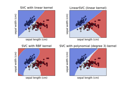
Verschiedene SVM-Klassifikatoren im Iris-Datensatz plotten