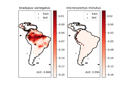
Kernel-Dichteschätzung von Artenverteilungen

Dies zeigt ein Beispiel für eine nachbarschaftsbasierte Abfrage (insbesondere eine Kernel-Dichteschätzung) auf Geodaten, unter Verwendung eines Ball Trees, der auf der Haversine-Distanzmetrik basiert – d.h. Distanzen über Punkte in Längen- und Breitengraden. Der Datensatz wird von Phillips et. al. (2006) [1] bereitgestellt. Sofern verfügbar, wird basemap verwendet, um die Küstenlinien und nationalen Grenzen Südamerikas zu plotten.

Dieses Beispiel führt kein Lernen der Daten durch (siehe Artenverbreitungsmodellierung für ein Beispiel der Klassifizierung basierend auf den Attributen in diesem Datensatz). Es zeigt lediglich die Kernel-Dichteschätzung beobachteter Datenpunkte in Geokoordinaten.

Die beiden Arten sind

• „Bradypus variegatus“, das Braunkehl-Faultier.

• „Microryzomys minutus“, auch bekannt als der kleine Waldreisratte, ein Nagetier, das in Peru, Kolumbien, Ecuador, Peru und Venezuela lebt.

Referenzen

[1]

„Maximum entropy modeling of species geographic distributions“ S. J. Phillips, R. P. Anderson, R. E. Schapire - Ecological Modelling, 190:231-259, 2006.

- computing KDE in spherical coordinates
- plot coastlines from coverage
- computing KDE in spherical coordinates
- plot coastlines from coverage

# Authors: The scikit-learn developers
# SPDX-License-Identifier: BSD-3-Clause

import matplotlib.pyplot as plt
import numpy as np

from sklearn.datasets import fetch_species_distributions
from sklearn.neighbors import KernelDensity

# if basemap is available, we'll use it.
# otherwise, we'll improvise later...
try:
    from mpl_toolkits.basemap import Basemap

    basemap = True
except ImportError:
    basemap = False


def construct_grids(batch):
    """Construct the map grid from the batch object

    Parameters
    ----------
    batch : Batch object
        The object returned by :func:`fetch_species_distributions`

    Returns
    -------
    (xgrid, ygrid) : 1-D arrays
        The grid corresponding to the values in batch.coverages
    """
    # x,y coordinates for corner cells
    xmin = batch.x_left_lower_corner + batch.grid_size
    xmax = xmin + (batch.Nx * batch.grid_size)
    ymin = batch.y_left_lower_corner + batch.grid_size
    ymax = ymin + (batch.Ny * batch.grid_size)

    # x coordinates of the grid cells
    xgrid = np.arange(xmin, xmax, batch.grid_size)
    # y coordinates of the grid cells
    ygrid = np.arange(ymin, ymax, batch.grid_size)

    return (xgrid, ygrid)


# Get matrices/arrays of species IDs and locations
data = fetch_species_distributions()
species_names = ["Bradypus Variegatus", "Microryzomys Minutus"]

Xtrain = np.vstack([data["train"]["dd lat"], data["train"]["dd long"]]).T
ytrain = np.array(
    [d.decode("ascii").startswith("micro") for d in data["train"]["species"]],
    dtype="int",
)
Xtrain *= np.pi / 180.0  # Convert lat/long to radians

# Set up the data grid for the contour plot
xgrid, ygrid = construct_grids(data)
X, Y = np.meshgrid(xgrid[::5], ygrid[::5][::-1])
land_reference = data.coverages[6][::5, ::5]
land_mask = (land_reference > -9999).ravel()

xy = np.vstack([Y.ravel(), X.ravel()]).T
xy = xy[land_mask]
xy *= np.pi / 180.0

# Plot map of South America with distributions of each species
fig = plt.figure()
fig.subplots_adjust(left=0.05, right=0.95, wspace=0.05)

for i in range(2):
    plt.subplot(1, 2, i + 1)

    # construct a kernel density estimate of the distribution
    print(" - computing KDE in spherical coordinates")
    kde = KernelDensity(
        bandwidth=0.04, metric="haversine", kernel="gaussian", algorithm="ball_tree"
    )
    kde.fit(Xtrain[ytrain == i])

    # evaluate only on the land: -9999 indicates ocean
    Z = np.full(land_mask.shape[0], -9999, dtype="int")
    Z[land_mask] = np.exp(kde.score_samples(xy))
    Z = Z.reshape(X.shape)

    # plot contours of the density
    levels = np.linspace(0, Z.max(), 25)
    plt.contourf(X, Y, Z, levels=levels, cmap=plt.cm.Reds)

    if basemap:
        print(" - plot coastlines using basemap")
        m = Basemap(
            projection="cyl",
            llcrnrlat=Y.min(),
            urcrnrlat=Y.max(),
            llcrnrlon=X.min(),
            urcrnrlon=X.max(),
            resolution="c",
        )
        m.drawcoastlines()
        m.drawcountries()
    else:
        print(" - plot coastlines from coverage")
        plt.contour(
            X, Y, land_reference, levels=[-9998], colors="k", linestyles="solid"
        )
        plt.xticks([])
        plt.yticks([])

    plt.title(species_names[i])

plt.show()

Verwandte Beispiele

Artenschutzmodellierung

Artenschutzmodellierung

Kernel-Dichteschätzung

Kernel-Dichteschätzung

SGD: Gewichtete Stichproben

SGD: Gewichtete Stichproben

Einfache 1D Kernel-Dichteschätzung

Einfache 1D Kernel-Dichteschätzung