Hinweis
Zum Ende springen, um den vollständigen Beispielcode herunterzuladen oder dieses Beispiel über JupyterLite oder Binder in Ihrem Browser auszuführen.
Feature Discretization#
Eine Demonstration der Feature-Discretization auf synthetischen Klassifikationsdatensätzen. Feature-Discretization zerlegt jedes Feature in eine Reihe von Bins, hier gleichmäßig in der Breite verteilt. Die diskreten Werte werden dann One-Hot-kodiert und einem linearen Klassifikator zugeführt. Diese Vorverarbeitung ermöglicht ein nicht-lineares Verhalten, obwohl der Klassifikator linear ist.
In diesem Beispiel stellen die ersten beiden Zeilen linear nicht trennbare Datensätze (Mond und konzentrische Kreise) dar, während die dritte annähernd linear trennbar ist. Bei den beiden linear nicht trennbaren Datensätzen erhöht die Feature-Discretization die Leistung linearer Klassifikatoren erheblich. Bei dem linear trennbaren Datensatz verringert die Feature-Discretization die Leistung linearer Klassifikatoren. Zum Vergleich werden auch zwei nicht-lineare Klassifikatoren gezeigt.
Dieses Beispiel sollte mit Vorsicht genossen werden, da die vermittelte Intuition nicht unbedingt auf reale Datensätze übertragbar ist. Insbesondere in hochdimensionalen Räumen können Daten leichter linear getrennt werden. Darüber hinaus erhöht die Verwendung von Feature-Discretization und One-Hot-Kodierung die Anzahl der Features, was bei wenigen Stichproben leicht zu Overfitting führen kann.
Die Diagramme zeigen Trainingspunkte in Vollfarben und Testpunkte halbtransparent. Unten rechts wird die Klassifikationsgenauigkeit auf dem Testdatensatz angezeigt.
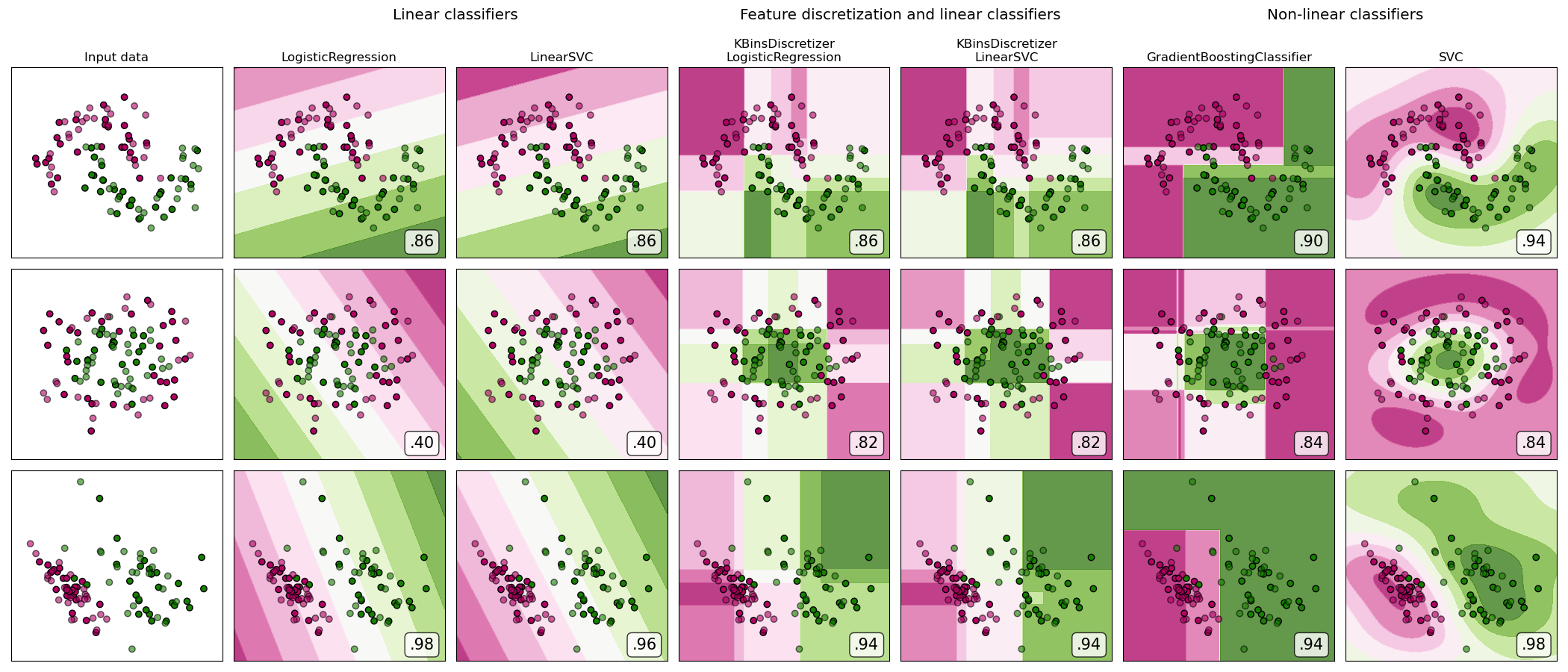
dataset 0
---------
LogisticRegression: 0.86
LinearSVC: 0.86
KBinsDiscretizer + LogisticRegression: 0.86
KBinsDiscretizer + LinearSVC: 0.86
GradientBoostingClassifier: 0.90
SVC: 0.94

dataset 1
---------
LogisticRegression: 0.40
LinearSVC: 0.40
KBinsDiscretizer + LogisticRegression: 0.82
KBinsDiscretizer + LinearSVC: 0.82
GradientBoostingClassifier: 0.84
SVC: 0.84

dataset 2
---------
LogisticRegression: 0.98
LinearSVC: 0.96
KBinsDiscretizer + LogisticRegression: 0.94
KBinsDiscretizer + LinearSVC: 0.94
GradientBoostingClassifier: 0.94
SVC: 0.98
# Authors: The scikit-learn developers
# SPDX-License-Identifier: BSD-3-Clause

import matplotlib.pyplot as plt
import numpy as np
from matplotlib.colors import ListedColormap

from sklearn.datasets import make_circles, make_classification, make_moons
from sklearn.ensemble import GradientBoostingClassifier
from sklearn.exceptions import ConvergenceWarning
from sklearn.linear_model import LogisticRegression
from sklearn.model_selection import GridSearchCV, train_test_split
from sklearn.pipeline import make_pipeline
from sklearn.preprocessing import KBinsDiscretizer, StandardScaler
from sklearn.svm import SVC, LinearSVC
from sklearn.utils._testing import ignore_warnings

h = 0.02  # step size in the mesh


def get_name(estimator):
    name = estimator.__class__.__name__
    if name == "Pipeline":
        name = [get_name(est[1]) for est in estimator.steps]
        name = " + ".join(name)
    return name


# list of (estimator, param_grid), where param_grid is used in GridSearchCV
# The parameter spaces in this example are limited to a narrow band to reduce
# its runtime. In a real use case, a broader search space for the algorithms
# should be used.
classifiers = [
    (
        make_pipeline(StandardScaler(), LogisticRegression(random_state=0)),
        {"logisticregression__C": np.logspace(-1, 1, 3)},
    ),
    (
        make_pipeline(StandardScaler(), LinearSVC(random_state=0)),
        {"linearsvc__C": np.logspace(-1, 1, 3)},
    ),
    (
        make_pipeline(
            StandardScaler(),
            KBinsDiscretizer(
                encode="onehot", quantile_method="averaged_inverted_cdf", random_state=0
            ),
            LogisticRegression(random_state=0),
        ),
        {
            "kbinsdiscretizer__n_bins": np.arange(5, 8),
            "logisticregression__C": np.logspace(-1, 1, 3),
        },
    ),
    (
        make_pipeline(
            StandardScaler(),
            KBinsDiscretizer(
                encode="onehot", quantile_method="averaged_inverted_cdf", random_state=0
            ),
            LinearSVC(random_state=0),
        ),
        {
            "kbinsdiscretizer__n_bins": np.arange(5, 8),
            "linearsvc__C": np.logspace(-1, 1, 3),
        },
    ),
    (
        make_pipeline(
            StandardScaler(), GradientBoostingClassifier(n_estimators=5, random_state=0)
        ),
        {"gradientboostingclassifier__learning_rate": np.logspace(-2, 0, 5)},
    ),
    (
        make_pipeline(StandardScaler(), SVC(random_state=0)),
        {"svc__C": np.logspace(-1, 1, 3)},
    ),
]

names = [get_name(e).replace("StandardScaler + ", "") for e, _ in classifiers]

n_samples = 100
datasets = [
    make_moons(n_samples=n_samples, noise=0.2, random_state=0),
    make_circles(n_samples=n_samples, noise=0.2, factor=0.5, random_state=1),
    make_classification(
        n_samples=n_samples,
        n_features=2,
        n_redundant=0,
        n_informative=2,
        random_state=2,
        n_clusters_per_class=1,
    ),
]

fig, axes = plt.subplots(
    nrows=len(datasets), ncols=len(classifiers) + 1, figsize=(21, 9)
)

cm_piyg = plt.cm.PiYG
cm_bright = ListedColormap(["#b30065", "#178000"])

# iterate over datasets
for ds_cnt, (X, y) in enumerate(datasets):
    print(f"\ndataset {ds_cnt}\n---------")

    # split into training and test part
    X_train, X_test, y_train, y_test = train_test_split(
        X, y, test_size=0.5, random_state=42
    )

    # create the grid for background colors
    x_min, x_max = X[:, 0].min() - 0.5, X[:, 0].max() + 0.5
    y_min, y_max = X[:, 1].min() - 0.5, X[:, 1].max() + 0.5
    xx, yy = np.meshgrid(np.arange(x_min, x_max, h), np.arange(y_min, y_max, h))

    # plot the dataset first
    ax = axes[ds_cnt, 0]
    if ds_cnt == 0:
        ax.set_title("Input data")
    # plot the training points
    ax.scatter(X_train[:, 0], X_train[:, 1], c=y_train, cmap=cm_bright, edgecolors="k")
    # and testing points
    ax.scatter(
        X_test[:, 0], X_test[:, 1], c=y_test, cmap=cm_bright, alpha=0.6, edgecolors="k"
    )
    ax.set_xlim(xx.min(), xx.max())
    ax.set_ylim(yy.min(), yy.max())
    ax.set_xticks(())
    ax.set_yticks(())

    # iterate over classifiers
    for est_idx, (name, (estimator, param_grid)) in enumerate(zip(names, classifiers)):
        ax = axes[ds_cnt, est_idx + 1]

        clf = GridSearchCV(estimator=estimator, param_grid=param_grid)
        with ignore_warnings(category=ConvergenceWarning):
            clf.fit(X_train, y_train)
        score = clf.score(X_test, y_test)
        print(f"{name}: {score:.2f}")

        # plot the decision boundary. For that, we will assign a color to each
        # point in the mesh [x_min, x_max]*[y_min, y_max].
        if hasattr(clf, "decision_function"):
            Z = clf.decision_function(np.column_stack([xx.ravel(), yy.ravel()]))
        else:
            Z = clf.predict_proba(np.column_stack([xx.ravel(), yy.ravel()]))[:, 1]

        # put the result into a color plot
        Z = Z.reshape(xx.shape)
        ax.contourf(xx, yy, Z, cmap=cm_piyg, alpha=0.8)

        # plot the training points
        ax.scatter(
            X_train[:, 0], X_train[:, 1], c=y_train, cmap=cm_bright, edgecolors="k"
        )
        # and testing points
        ax.scatter(
            X_test[:, 0],
            X_test[:, 1],
            c=y_test,
            cmap=cm_bright,
            edgecolors="k",
            alpha=0.6,
        )
        ax.set_xlim(xx.min(), xx.max())
        ax.set_ylim(yy.min(), yy.max())
        ax.set_xticks(())
        ax.set_yticks(())

        if ds_cnt == 0:
            ax.set_title(name.replace(" + ", "\n"))
        ax.text(
            0.95,
            0.06,
            (f"{score:.2f}").lstrip("0"),
            size=15,
            bbox=dict(boxstyle="round", alpha=0.8, facecolor="white"),
            transform=ax.transAxes,
            horizontalalignment="right",
        )


plt.tight_layout()

# Add suptitles above the figure
plt.subplots_adjust(top=0.90)
suptitles = [
    "Linear classifiers",
    "Feature discretization and linear classifiers",
    "Non-linear classifiers",
]
for i, suptitle in zip([1, 3, 5], suptitles):
    ax = axes[0, i]
    ax.text(
        1.05,
        1.25,
        suptitle,
        transform=ax.transAxes,
        horizontalalignment="center",
        size="x-large",
    )
plt.show()
Gesamtlaufzeit des Skripts: (0 Minuten 3,436 Sekunden)
Verwandte Beispiele
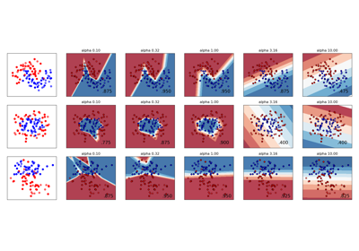
Variierende Regularisierung im Multi-Layer Perceptron
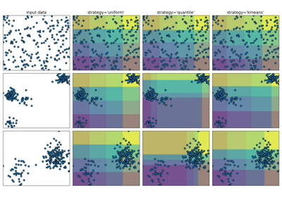
Demonstration der verschiedenen Strategien von KBinsDiscretizer
Gauß-Prozess-Klassifikation (GPC) auf dem Iris-Datensatz